
Milvus User Guide
# Database
Milvus introduces a database layer above collections, providing a more efficient way to manage and organize your data while supporting multi-tenancy.
# What is a database
In Milvus, a database serves as a logical unit for organization and managing data. To enhance data security and achieve multi-tenancy, you can create multiple databases to logically isolate data for different applications or tenants. For example, you create a database to store the data of user A and another database for user B.
# Create database
You can use the Milvus RESTful API or SDKs to create data programmatically.
from pymilvus import MilvusClient

client = MilvusClient(
    uri="http://localhost:19530",
    token="root:Milvus"
)

client.create_database(
    db_name="my_database_1"
)
2
3
4
5
6
7
8
9
10
You can also set properties for the database when you create it. The following example sets the number of replicas of the database.
client.create_database(
    db_name="my_database_2",
    properties={
        "database.replica.number": 3
    }
)
2
3
4
5
6
# View database
You can use the Milvus RESTful API or SDKs to list all existing databases and view their details.
# List all existing databases
client.list_databases()

# Output
# ['default', 'my_database_1', 'my_database_2']

# Check database details
client.describe_database(
    db_name="default"
)

# Output
# {"name": "default"}
2
3
4
5
6
7
8
9
10
11
12
13
# Manage database properties
Each database has its own properties, you can set the properties of a database when you create the database as described in Create database or you can alter and drop the properties of any existing database.
The following table lists possible database properties.
| Property Name | Type | Property Description |
|---|---|---|
database.replica.number | integer | The number of replicas for the specified database. |
database.resource_groups | string | The names of the resource groups associated with the specified database in a comma-separated list. |
database.diskQuota.mb | integer | The maximum size of the disk space for the specified database, in megabytes(MB). |
database.max.collections | integer | The maximum number of collections allowed in the specified database. |
database.force.deny.writing | boolean | Whether to force the specified database to deny writing operations. |
database.force.deny.reading | boolean | Whether to force the specified database to deny reading operations. |
# Alter database properties
You can alter the properties of an existing database as follows. The following example limits the number of collections you can create in the database.
client.alter_database_properties(
    db_name="my_database_1",
    properties={
        "database.max.collections": 10
    }
)
2
3
4
5
6
# Drop database properties
You can also reset a database property by dropping it as follows. The following example removes the limit on the number of collections you can create in the database.
client.drop_database_properties(
    db_name="my_database_1",
    property_keys=[
        "database.max.collections"
    ]
)
2
3
4
5
6
# Use database
You can switch from one database to another without disconnecting from Milvus.
NOTE
RESTful API does not support this operation.
client.use_database(
    db_name="my_database_2"
)
2
3
# Drop database
Once a database is no longer needed, you can drop the database. Note that:
- Default databases cannot be dropped.
- Before dropping a database, you need to drop all collections in the database first.
You can use the Milvus RESTful API or SDKs to create data programmatically.
client.drop_database(
    db_name="my_database_2"
)
2
3
# FAQ
# How do i manage permissions for a database?
Milvus uses Role-Based Access Control (RBAC) to manage permissions. You can create roles with specific privileges and assign them to users, thus controlling their access to different databases. For more details, refer to the RBAC documentation.
# Are there any quota limitations for a database?
Yes, Milvus allows you to set quota limitations for a database, such as the maximum number of collections. For a comprehensive list of limitations, please refer to the Milvus Limits documentation.
# Collections
# Collection Explained
On Milvus, you can create multiple collections to manage your data, and insert your data as entities into the collections. Collection and entity are similar to tables and records in relational databases. This page helps you to learn about the collection and related concepts.
# Collection
A collection is a two-dimensional table with fixed columns and variant rows. Each column represents a field, and each row represents an entity.
The following chart shows a collection with eight columns and six entities.
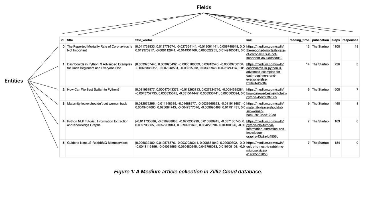
# Schema and Fields
When describing an object, we usually mention its attributes, such as size, weight, and position. You can use these attributes as fields in a collection. Each field has various constraining properties, such as the data type and the dimensionality of a vector field. You can form a collection schema by creating the fields and defining their order. For possible applicable data types, refer to Schema Explained.
You should include all schema-defined fields in the entities to insert. To make some of them optional, consider enabling dynamic field. For details, refer to Dynamic Field.
- Making them nullable or setting default values: For details on how to make a field nullable or set the default value, refer to Nullable & Default.
- Enabling dynamic field: For details on how to enable and use the dynamic field, refer to Dynamic Field.
# Primary key and AutoId
Similar to the primary field in a relational database, a collection has a primary field to distinguish an entity from others. Each value in the primary field is globally unique and corresponds to one specific entity.
As shown in the above chart, the field named id serves as the primary field, and the first ID 0 corresponds to an entity titled The Mortality Rate of Coronavirus is Not Important. There will not be any other entity that has the primary field of 0.
A primary field accepts only integers or strings. When inserting entities, you should include the primary field values by default. However, if you have enabled AutoId upon collection creation, Milvus will generate those values upon data insertion. In such a case, exclude the primary field values from the entities to be inserted.
For more information, please refer to Primary Field & AutoId.
# Index
Creating indexes on specific fields improves search efficiency. You are advised to create indexes for all the fields your service relies on, among which indexes on vector fields are mandatory.
# Entity
Entities are data records that share the same set of fields in a collection. The values in all fields of the same row comprise an entity.
You can insert as many entities as you need into a collection. However, as the number of entities mounts, the memory size it takes also increases, affecting search performance.
For more information, refer to Schema Explained.
# Load and Release
Loading a collection is the prerequisite to conducting similarity searches and queries in collections. When you load a collection, Milvus loads all index files and the raw data in each field into memory for fast response to searches and queries.
Searches and queries are memory-intensive operations. To save the cost, you are advised to release the collections that are currently not in use.
For more details, refer to Load & Release.
# Search and Query
Once you create indexes and load the collection, you can start a similarity search by feeding one or several query vectors. For example, when receiving the vector representation of your query carried in a search request, Milvus uses the sepcified metric type to measure the similarity between the query vector and those in the target collection before returning those that are semantically similar to the query.
You can also include metadata filtering within searches and queries to improve the relevancy of the results. Note that, metadata filtering conditions are mandatory in queries but optional in searches.
For details on applicable metric types, refer to Metric Types.
For more information about searches and queries, refer to the articles in the Search & Rerank chapter, among which, basic features are:
- Basic ANN Search
- Filtered Search
- Range Search
- Grouping Search
- Hybrid Search
- Search Iterator
- Query
- Full Text Search
- Text Match
In addition, Milvus also provides enhancements to improve search performance and efficiency. They are disabled by default, and you can enable and use them according to your service requirements. They are
# Partition
Partitions are subsets of a collection which share the same field set with its parent collection, each containing a subset of entities.
By allocating entities into different partitions, you can create entity groups. You can conduct searches and queries in sepcific partitions to have Milvus ignore entities in other partitions, and improve search efficiency.
For details, refer to Manage Partitions.
# Shard
Shards are horizontal slices of a collection. Each shard corresponds to a data input channel. Every collection has a shard by default. You can set the appropriate number of shards when creating a collection based on the expected throughput and the volume of the data to insert into the collection.
For details on how to set the shard number, refer to Create Collection.
# Alias
You can create aliases for your collections. A collection can have serveral aliases, but collections cannot share an alias. Upon receiving a request against a collection, Milvus locates the collection based on the provided name. If the collection by the provided name does not exist, Milvus continues locating the provided name as an alias. You can use collection aliases to adapt your code to different scenarios.
For more details, refer to Manage Aliases.
# Function
You can set functions for Milvus to derive fields upon collection creation. For example, the full-text search function uses the user-defined function to derive a sparse vector field from a specific varchar field. For more information on full-text search, refer to Full Text Search.
# Consistency Level
Distributed database systems usually use the consistency level to define the data sameness across data nodes and replicas. You can set separate consistency levels when you create a collection or conduct similarity searches within the collection. The applicable consistency levels are Strong, Bounded Staleness, Session, and Eventually.
For details on these consistency levels, refer to Consistency Level.
# Create Collection
You can create a collection by defining its schema, index parameters, metric type, and whether to load it upon creation. This page introduces how to create a collection from scratch.
# Overview
A collection is a two-dimensional table with fixed columns and variant rows. Each column represents a field, and each row represents an entity. A schema is required to implement such structural data management. Every entity to insert has to meet the constraints defined in the schema.
You can determine every aspect of a collection, including its schema, index parameters, metric type, and whether to load it upon creation to ensure that the collection fully meets your requirements.
To create a collection, you need to:
# Create Schema
A schema defines the data structure of a collection. When creating a collection, you need to design the schema based on your requirements. For details, refer to Schema Explained.
The following code snippets create a schema with the enabled dynamic field and three mandatory fields named my_id, my_vector, and my_varchar.
NOTE
You can set default values for any scalar field and make it nullable. For details, refer to Nullable & Default.
# 3. Create a collection in customized setup mode
from pymilvus import MilvusClient, DataType

client = MilvusClient(
    uri="http://localhost:19530",
    token="root:Milvus"
)

# 3.1 Create schema
schema = MilvusClient.create_schema(
    auto_id=False,
    enable_dynamic_field=True
)

# 3.2 Add fields to schema
schema.add_field(field_name="my_id", datatype=DataType.INT64, is_primary=True)
schema.add_field(field_name="my_vector", datatype=DataType.FLOAT_VECTOR, dim=5)
schema.add_field(field_name="my_varchar", datatype=DataType.VARCHAR, max_length=512)
2
3
4
5
6
7
8
9
10
11
12
13
14
15
16
17
18
# (Optional) Set Index Parameters
Creating an index on a specific field accelerates the search against this field. An index records the order of entities within a collection. As shown in the following code snippets, you can use metric_type and index_type to select appropriate ways for Milvus to index a field and measure similarities between vector embeddings.
On Milvus, you can use AUTOINDEX as the index type for all vector field, and one of COSINE, L2 and IP as the metric type based on your needs.
As demonstrated in the above code snippets, you need to set both the index type and metric type for vector fields and only the index type for the scalar fields. Indexes are mandatory for vector fields, and you are advised to create indexes on scalar fields frequently used in filtering conditions.
For details, refer to Index Vector Fields and Index Scalar Fields.
# 3.3 Prepare index parameters
index_params = client.prepare_index_params()

# 3.4 Add indexes
index_params.add_index(
    field_name="my_id",
    index_type="AUTOINDEX"
)

index_params.add_index(
    field_name="my_vector",
    index_type="AUTOINDEX",
    metric_type="COSINE"
)
2
3
4
5
6
7
8
9
10
11
12
13
14
# Create a Collection
If you have created a collection with index parameters, Milvus automatically loads the collection upon its creation. In this case, all fields mentioned in the index parameters are indexed.
The following code snippets demonstrate how to create the collection with index parameters and check its load status.
# 3.5 Create a collection with the index loaded simultaneously
client.create_collection(
    collection_name="customized_setup_1",
    schema=schema,
    index_params=index_params
)

res = client.get_load_state(
    collection_name="customized_setup_1"
)

print(res)

# Output
#
# {
#     "state": "<LoadState: Loaded>"
# }
2
3
4
5
6
7
8
9
10
11
12
13
14
15
16
17
18
You can also create a collection without any index parameters and add them afterward. In this case, Milvus does not load the collection upon its creation.
The following code snippet demonstrates how to create a collection without an index, and the load status of the collection remains uploaded upon creation.
# 3.6 Create a collection and index it separately
client.create_collection(
    collection_name="customized_setup_2",
    schema=schema,
)

res = client.get_load_state(
    collection_name="customized_setup_2"
)

print(res)

# Output
#
# {
#     "state": "<LoadState: Notload>"
# }
2
3
4
5
6
7
8
9
10
11
12
13
14
15
16
17
# Set Collection Properties
You can set properties for the collection to create to make it fit into your service. The applicable properties are as follows.
# Set Shard Number
Shards are horizontal slices of a collection, and each shard corresponds to a data input channel. By default, every collection has one shard. You can specify the number of shards when creating a collection to better suit your data volume and workload.
As a general guideline, consider the following when setting the number of shards:
- Data size: A common practice is to have one shard for every 200 million entities. You can also estimate based on the total data size, for example, adding one shard for every 100 GB of data you plan to insert.
- Stream node utilization: If your Milvus instance has multiple stream nodes, using multiple shards is recommended. This ensure that the data insertion workload is distributed across all available stream nodes, preventing some from being idle while others are overloaded.
The following code snippet demonstrates how to set the shard number when you create a collection.
# With shard number
client.create_collection(
    collection_name="customized_setup_3",
    schema=schema,
    num_shards=1
)
2
3
4
5
6
# Enable mmap
Milvus enables mmap on all collection by default, allowing Milvus to map raw field data int memory instead of fully loading them. This reduces memory footprints and increases collection capacity. For details on mmap, refer to Use mmap.
# With mmap
client.create_collection(
    collection_name="customized_setup_4",
    schema=schema,
    enable_mmap=False
)
2
3
4
5
6
# Set Collection TTL
If the data in a collection needs to be dropped for a specific period, consider setting its Time-To-Live(TTL) in seconds. Once the TTL times out, Milvus deletes entities in the collection. The deletion is asynchronous, indicating that searches and queries are still possible before the deletion is complete.
The following code snippet sets the TTL to one day (86400 seconds). You are advised to set the TTL to a couple of days at minimum.
# With TTL
client.create_collection(
    collection_name="customized_setup_5",
    schema=schema,
    properties={
        "collection.ttl.seconds": 86400
    }
)
2
3
4
5
6
7
8
# Set Consistency Level
When creating a collection, you can set the consistency level for searches and queries in the collection. You can also change the consistency level of the collection during a specific search or query.
# With consistency level
client.create_collection(
    collection_name="customized_setup_6",
    schema=schema,
    consistency_level="Bounded",
)
2
3
4
5
6
For more on consistency levels, see Consistency Level.
# Enable Dynamic Field
The dynamic field in a collection is a reserved JavaScript Object Notation (JSON) field named $meta. Once you have enabled this field, Milvus saves all non-schema-defined fields carried in each entity and their values as key-value pairs in the reserved field.
For details on how to use the dynamic field, refer to Dynamic Field.
# View Collections
You can obtain the name list of all the collections in the currently dataase, and check the details of a specific collection.
# List Collections
The following example demonstrates how to abtain the name list of all collections in the currently connected database.
from pymilvus import MilvusClient, DataType

client = MilvusClient(
    uri="http://localhost:19530",
    token="root:Milvus"
)

res = client.list_collections()

print(res)
2
3
4
5
6
7
8
9
10
If you have already created a collection named quick_setup, the result of the above example should be similar to the following.
["quick_setup"]
# Describe Collection
You can also obtain the details of a specific collection. The following example assumes that you have already created a collection named quick_setup.
res = client.describe_collection(
    collection_name="quick_setup"
)

print(res)
2
3
4
5
The result of the above example should be similar to the following.
{
    'collection_name': 'quick_setup',
    'auto_id': False,
    'num_shards': 1,
    'description': '',
    'fields': [
        {
            'field_id': 100,
            'name': 'id',
            'description': '',
            'type': <DataType.INT64: 5>,
            'params': {},
            'is_primary': True
        },
        {
            'field_id': 101,
            'name': 'vector',
            'description': '',
            'type': <DataType.FLOAT_VECTOR: 101>,
            'params': {'dim': 768}
        }
    ],
    'functions': [],
    'aliases': [],
    'collection_id': 456909630285026300,
    'consistency_level': 2,
    'properties': {},
    'num_partitions': 1,
    'enable_dynamic_field': True
}
2
3
4
5
6
7
8
9
10
11
12
13
14
15
16
17
18
19
20
21
22
23
24
25
26
27
28
29
30
31
# Modify Collection
You can rename a collection or change its settings. This page focuses on how to modify a collection.
# Rename Collection
You can rename a collection as follows.
from pymilvus import MilvusClient

client = MilvusClient(
    uri="http://localhost:19530",
    token="root:Milvus"
)

client.rename_collection(
    old_name="my_collection",
    new_name="my_new_collection"
)
2
3
4
5
6
7
8
9
10
11
# Set Collection Properties
The following code snippet demonstrates how to set collection TTL.
from pymilvus import MilvusClient

client.alter_collection_properties(
    collection_name="my_collection",
    properties={"collection.ttl.seconds": 60}
)
2
3
4
5
6
The applicable collection properties are as follows:
| Property | When to Use |
|---|---|
collection.ttl.seconds | If the data of a collection needs to be deleted after a specific period, consider setting its Time-To-Live(TTL) in seconds. Once the TTL times out, Milvus deletes all entities from the collection. THe deletion is asynchronous, indicating that searches and queries are still possible before the deletion is complete. For details, refer to Set Collection TTL. |
mmap.enabled | Memory mapping (Mmap) enables direct memory access to large files on disk, allowing Milvus to store indexes and data in both memory and hard drives. This approach helps optimize data placement policy based on access frequency, expanding storage capacity for collections without impacting search performance. For details, refer to Use mmap |
partitionkey.isolation | With Partition Key Isolation enabled, Milvus groups entities based on the Partition Key value and creates a separate index for each of these groups. Upon receiving a search request, Milvus locates the index based on the Partition Key value specified in the filtering condition and restricts the search scope within the entities included in the index, thus avoiding scanning irrelevant entities durint the search geatly enhancing the search performance. For details, refer to Use Partition Key Isolation. |
# Drop Collection Properties
You can also reset a collection property by dropping it as follows.
client.drop_collection_properties(
    collection_name="my_collection",
    property_keys=[
        "collection.ttl.seconds"
    ]
)
2
3
4
5
6
# Load & Release
Loading a collection is the prerequisite to conducting similarity searches and queries in collections. This page focuses on the procedures for loading and releasing a collection.
# Load Collection
When you load a collection, Milvus loads the index files and the raw data of all fields into memory for rapid response to searches and queries. Entities inserted after a collection load are automatically indexed and loaded.
The following code snippets demonstrate how to load a collection.
from pymilvus import MilvusClient

client = MilvusClient(
    uri="http://localhost:19530",
    token="root:Milvus"
)

# 7. Load the collection
client.load_collection(
    collection_name="my_collection"
)

res = client.get_load_state(
    collection_name="my_collection"
)

print(res)

# Output
#
# {
#     "state": "<LoadState: Loaded>"
# }
2
3
4
5
6
7
8
9
10
11
12
13
14
15
16
17
18
19
20
21
22
23
# Load Specific Fields
Milvus can load only the fields involved in searches and queries, reducing memory usage and improving search performance.
NOTE
Partial collection loading is currently in beta and not recommanded for production use.
The following code snippet assumes that you have created a collection named my_collection, and there are two fields named my_id and my_vector in the collection.
client.load_collection(
    collection_name="my_collection",
    load_fields=["my_id", "my_vector"], # Load only the specified fields
    skip_load_dynamic_field=True # Skip loading the dynamic field
)

res = client.get_load_state(
    collection_name="my_collection"
)

print(res)

# Output
# {
#     "state": "<LoadState: Loaded>"
# }
2
3
4
5
6
7
8
9
10
11
12
13
14
15
16
If you choose to load specific fields, it is worth noting that only the fields included in load_fields can be used as filters and output fields in searches and queries. You should always include the names of the primary field and at least one vector field in load_fields.
You can also use skip_load_dynamic_field to determine whether to load the dynamic field. The dynamic field is a reserved JSON field named $meta and saves all non-schema-defined fields and their values in key-value pairs. When loading the dynamic field, all keys in the fields are loaded and availabe for filtering and output. If all keys in the dynamic field are not involved in metadata filtering and output, set skip_load_dynamic_field to True.
To load more fields after the collection load, you need to release the collection first to avoid possible errors prompted because of index changes.
# Release Collection
Searches and queries are memory-intensive operations. To save the cost, you are advised to release the collections that are currently not in use.
The following code snippet demonstrates how to release a collection.
# 8. Release the collection
client.release_collection(
    collection_name="my_collection"
)

res = client.get_load_state(
    collection_name="my_collection"
)

print(res)

# Output
# {
#     "state": "<LoadState: Notload>"
# }
2
3
4
5
6
7
8
9
10
11
12
13
14
15
# Set Collection TTL
Once data is inserted into a collection, it remains there by default. However, in some scenarios, you may want to remove or clean up data after a certain period. In such cases, you can configure the collection's Time-to-Live (TTL) property so that Milvus automatically deletes the data once the TTL expires.
# Overview
Time-to-Live (TTL) is commonly used in databases for scenarios where data should only remain valid or accessible for a certain period after any insertion or modification. Then, the data can be automatically removed.
For instance, if you ingest data daily but only need to retain records for 14 days, you can configure Milvus to automatically remove any data older than that by setting the collection's TTL to 14 * 14 * 3600 = 1209600 seconds. This ensure that only the most of recent 14 days' worth of data remain in the collection.
NOTE
Expired entities will not appear in any search or query results. However, they may stay in the storage until the subsequent data compaction, which should be carried out within the next 24 hours.
You can control when to trigger the data compaction by setting the dataCoord.compaction.expiry.tolerance configuraiton item in your Milvus configuration file.
This configuration item defaults to -1, indicating that the existing data compaction interval applies. However, when you can change its value to a positive integer, like 12, data compaction will be triggered the specified number of hours after any entities become expired.
The TTL property in a Milvus collection is specified as an integer in seconds. Once set, any data that surpasses its TTL will be automatically deleted from the collection.
Because the deletion process is asynchronous, data might not be removed from search results exactly once the specified TTL has elapsed. Instead, there may be a delay, as the removal depends on the garbage collection (GC) and compaction processes, which occur at non-deterministic intervals.
# Set TTL
You can set the TTL property when you:
# Set TTL when creating a collection
The following code snippet demonstrates how to set the TTL property when you create a collection.
from pymilvus import MilvusClient

# With TTL
client.create_collection(
    collection_name="my_collection",
    schema=schema,
    properties={
        "collection.ttl.seconds": 1209600
    }
)
2
3
4
5
6
7
8
9
10
# Set TTL for an existing collection
The following code snippet demonstrates how to alter the TTL property in an existing collection.
client.alter_collection_properties(
    collection_name="my_collection",
    properties={"collection.ttl.seconds": 1209600}
)
2
3
4
# Drop TTL setting
If you decide to keep the data in a collection indefinitely, you can simply drop the TTL setting from that collection.
client.drop_collection_properties(
    collection_name="my_collection",
    property_keys=["collection.ttl.seconds"]
)
2
3
4
# Set Consistency Level
As a distributed vector database, Milvus offers multiple levels of consistency to ensure that each node or replica can access the same data during read and write operations. Currenty, the supported levels of consistency include Strong, Bounded, Eventually, and Session, with Bounded being the default level of consistency used.
# Overview
Milvus is a system that separates storage and computation. In this system, DataNodes are responsible for the persistence of data and ultimately store it in distributed object storage such as MinIO/S3. QueryNode handle computational tasks like Search. These tasks involve processing both batch data and streaming data. Simply put, batch data can be understood as data that has already been stored in object storage while streaming data refers to data that has not yet been stored in object storage. Due to network latency, QueryNodes often do not hold the most recent streaming data. Without additional safeguards, performing Search directly on streaming data may result in the loss of many uncommitted data points, affecting the accuracy of search results.
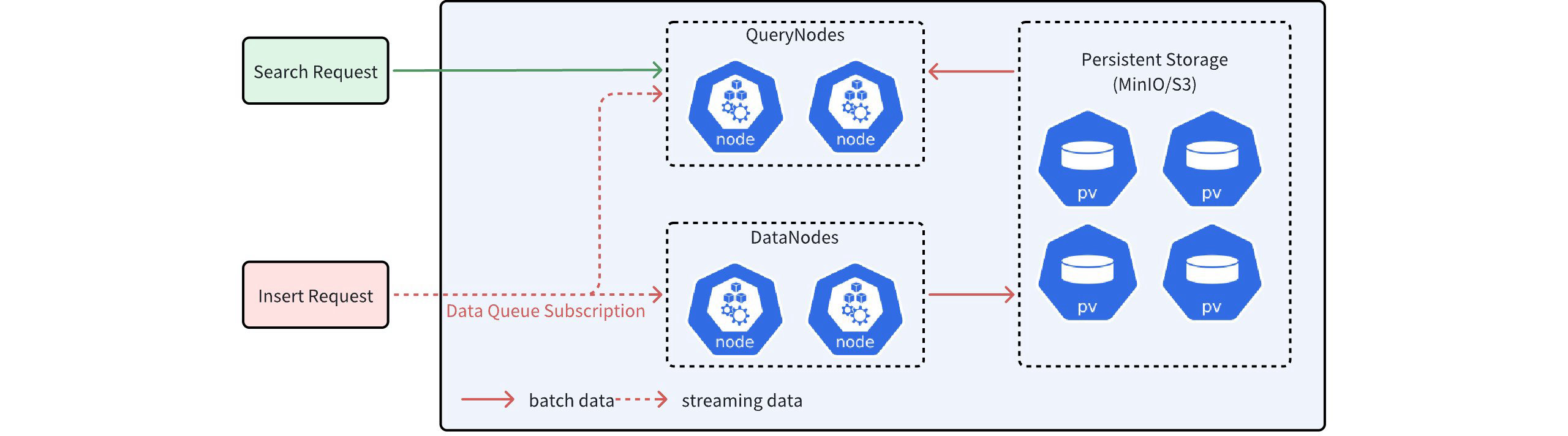
As shown in the figure above, QueryNodes can receive both streaming data and batch data simultaneously after receiving a Search request. However, due to network latency, the streaming data obtained by QueryNodes may be incomplete.
To address this issue, Milvus timestamps each record in the data queue and continuously inserts synchronization timestamps into the data queue. Whenever a synchronization timestamp (syncTs) is received, QueryNodes sets it as the ServiceTime, meaning that QueryNodes can see all data prior to that Service Time. Based on the ServiceTime, Milvus can provide guarantee timestamps (GuaranteeTs) to meet different user requirements for consistency and availability. Users can inform QueryNodes of the need to include data prior to a specified point in time in the search scope by specifying GuaranteeTs in their requests.
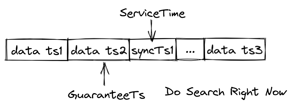
As shown in the figure above, if GuaranteeTs is less than ServiceTime, it means that all data before the specified time point has been fully written to disk, allowing QueryNodes to immediately perform the Search operation. When GuaranteeTs is greater than ServiceTime, QueryNodes must wait until ServiceTime exceeds GuaranteeTs before they can execute the Search operation.
Users need to make a trade-off between query accuracy and query latency. If users have high consistency requirements and are not sensitive to query latency, they can set GuaranteeTs to a value as large as possible; if users wish to receive search results quickly and are more tolerant of query accuracy, then GuaranteeTs can be set to a smaller value.
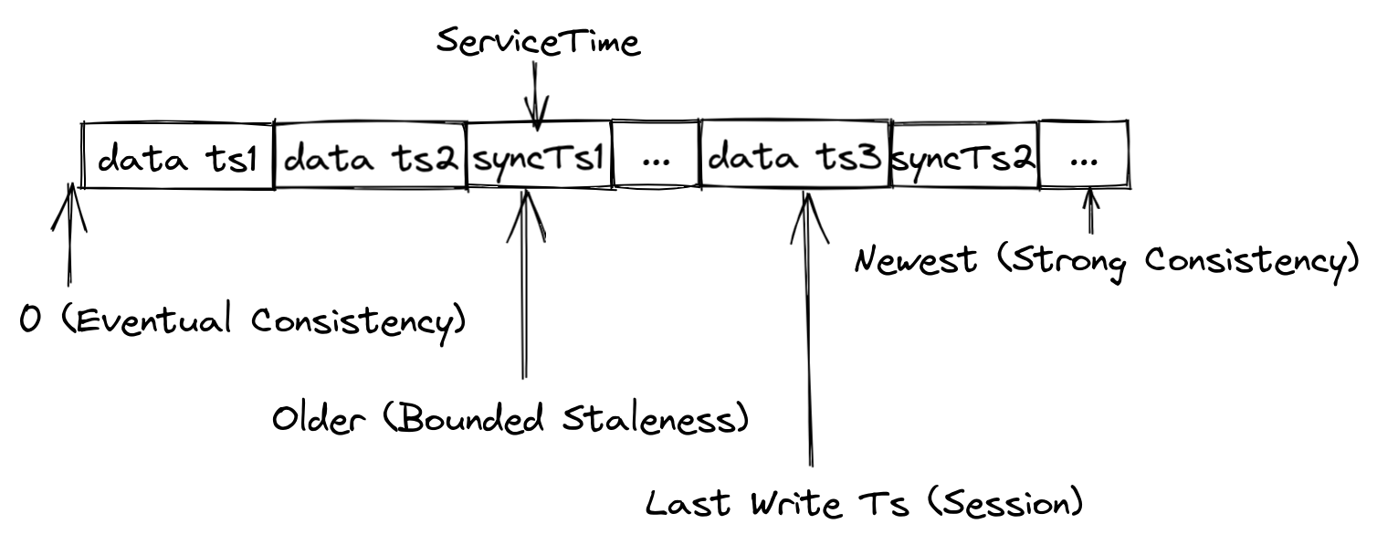
Milvus provides four types of consistency levels with different GuaranteeTs.
- Strong: The latest timestamp is used as the GuaranteeTs, and QueryNodes have to wait until the ServiceTime meets the GuaranteeTs before executing Search requests.
- Eventual: The GuaranteeTs is set to an extremely small value, such as 1, to avoid consistency checks so that QueryNodes can immediately execute Search requests upon all batch data.
- Bounded Staleness: The GuranteeTs is set to a time point earlier than the latest timestamp to make QueryNodes to perform searches with a tolerance of certain data loss.
- Session: The latest time point at which the client inserts data is used as the GuaranteeTs so that QueryNodes can perform searches upon all the data inserted by the client.
Milvus uses Bounded Staleness as the default consistency leve. If the GuaranteeTs is left unspecified, the latest ServiceTime is used as the GuaranteeTs.
# Set Consistency Level
You can set different consistency levels when you create a collection as well as perform searches and queries.
# Set Consistency Level upon Creating Collection
When creating a collection, you can set the consistency level for the searches and queries within the collection. The following code example sets the consistency level to Strong.
client.create_collection(
    collection_name="my_collection",
    schema=schema,
    consistency_level="Bounded"
)
2
3
4
5
Possible values for the consistency_level parameter are Strong, Bounded, Eventually, and Session.
# Set Consistency Level in Search
You can always change the consistency level for a specific search. The following code example sets the consistency level back to the Bounded. The change applies only to the current search request.
res = client.search(
    collection_name="my_collection",
    data=[query_vector],
    limit=3,
    search_params={"metric_type": "IP"},
    consistency_level="Bounded",
)
2
3
4
5
6
7
This parameter is also available in hybrid searches and the search iterator. Possible values for the consistency_level parameter are Strong, Bounded, Eventually, Session.
# Set Consistency Level in Query
You can always change the consistency level for a specific search. The following code example sets the consistency level to the Eventually. THe setting applies only to the current query request.
res = client.query(
    collection_name="my_collection",
    filter="color like \"red%\%",
    output_fields=["vector", "color"],
    limit=3,
    consistency_level="Eventually",
)
2
3
4
5
6
7
This parameter is also available in query iterator. Possible values for the consistency_level parameter are Strong, Bounded, Eventually, Session.
# Manage Partitions
A partition is a subset of a collection. Each partition shares the same data structure with its parent collection but contains only a subset of the data in the collection. This page helps you understand how to manage partitions.
# Overview
When creating a collection, Milvus also creates a partition named _default in the collection. If you are not going to add any other partitions, all entities inserted into the collection go into the default partition, and all searches and queries are also carried out within the default partition.
You can add more partitions and insert entities into them based on certain criteria. Then you can restrict your searches and queries within certain partitions, improving search performance.
A collection can have a maximum of 1024 partitions.
NOTE
The Partition Key feature is a search optimization based on partitions and allows Milvus to distribute entities into different partitions based on the values in a specific scalar field. This feature helps implement partition-oriented multi-tenancy and improves search performance.
This feature will not be discussed on this page. To find more, refer to Use Partition Key.
# List Partitions
When creating a collection, Milvus also creates a partition named _default in the collection. You can list the partitions in a collection as follows.
from pymilvus import MilvusClient

client = MilvusClient(
    uri="http://localhost:19530",
    token="root:Milvus"
)

res = client.list_partitions(
    collection_name="my_collection"
)

print(res)

# Output
#
# ["_default"]
2
3
4
5
6
7
8
9
10
11
12
13
14
15
16
# Create Partition
You can add more partitions to the collection and insert entities into these partitions based on certain criteria.
client.create_partition(
    collection_name="my_collection",
    partition_name="partitionA"
)

res = client.list_partitions(
    collection_name="my_collection"
)

print(res)

# Output
#
# ["_default", "partitionA"]
2
3
4
5
6
7
8
9
10
11
12
13
14
# Check for a Specific Partition
The following code snippets demonstrate how to check whether a partition exists in a specific collection.
res = client.has_partition(
    collection_name="my_collection",
    partition_name="partitionA"
)

print(res)

# Output
#
# True
2
3
4
5
6
7
8
9
10
# Load and Release Partitions
You can separately load or release one or certain partitions.
# Load Partitions
You can separately load specific partitions in a collection. It is worth noting that load status of a collection stays unloaded if there is an unloaded partition in the collection.
client.load_partitions(
    collection_name="my_collection",
    partition_names=["partitionA"]
)

res = client.get_load_state(
    collection_name="my_collection",
    partition_name="partitionA"
)

print(res)

# Output
#
# {
#     "state": "<LoadState: Loaded>"
# }
2
3
4
5
6
7
8
9
10
11
12
13
14
15
16
17
# Release Partitions
You can also release specific partitions.
client.release_partitions(
    collection_name="my_collection",
    partition_names=["partitionA"]
)

res = client.get_load_state(
    collection_name="my_collection",
    partition_name="partitionA"
)

print(res)

# Output
#
# {
#     "state": "<LoadState: NotLoaded>"
# }
2
3
4
5
6
7
8
9
10
11
12
13
14
15
16
17
# Data Operations Within Partitions
# Insert and Delete Entities
You can perform insert, upsert, and delete operations in specific operations. For details, refer to
# Search and Query
You can conduct searches and queries within specific partitions. For details, refer to
# Drop Partition
You can drop partitions that are no longer needed. Before dropping a partition, ensure that the partition has been released.
client.release_partitions(
    collection_name="my_collection",
    partition_names=["partitionA"]
)

client.drop_partition(
    collection_name="my_collection",
    partition_name="partitionA"
)

res = client.list_partitions(
    collection_name="my_collection"
)

print(res)

# ["_default"]
2
3
4
5
6
7
8
9
10
11
12
13
14
15
16
17
# Manage Aliases
In Milvus, an alias is a secondary, mutable name for a collection. Using aliases provides a layer of abstraction that allows you to dynamically switch between collections without modifying your application code. This is particularly useful in production environments for seamless data updates, A/B testing, and other operational tasks.
This page demonstrates how to create, list, reassign, and drop collection aliases.
# Why Use an Alias?
The primary benefit of using an alias is to decouple your client application from a specific, physical collection name.
Imagine you have a live application that queries a collection named prod_data. When you need to update the underlying data, you can perform the update without any service interruption. The workflow would be:
- Create a New Collection: Create a new collection, for instance,
prod_data_v2. - Prepare Data: Load and index the new data in
prod_data_v2. - Switch the Alias: Once the new collection is ready for service, atomically reassign the alias
prod_datafrom the old collection toprod_data_v2.
Your application continues to send requests to the alias prod_data, experiencing zero downtime. This mechanism enables seamless updates and simplifies operations like blue-green deployments for your vector search service.
Key Properties of Aliases:
- A collection can have multiple aliases.
- An alias can only point to one collection at a time.
- When processing a request, Milvus first checks if a collection with the provided name exists. If not, it then checks if the name is an alias for a collection.
# Create Alias
The following code snippet demonstrates how to create an alias for a collection.
from pymilvus import MilvusClient

client = MilvusClient(
    uri="http://localhost:19530",
    token="root:Milvus"
)

# 9. Manage aliases
# 9.1. Create aliases
client.create_alias(
    collection_name="my_collection_1",
    alias="bob"
)

client.create_alias(
    collection_name="my_collection_1",
    alias="alice"
)
2
3
4
5
6
7
8
9
10
11
12
13
14
15
16
17
18
# List Aliases
The following code snippet demonstrates the procedure to list the aliases allocated to a specific collection.
# 9.2. List aliases
res = client.list_aliases(
    collection_name="my_collection_1"
)

print(res)

# Output
#
# {
#     "aliases": [
#         "bob",
#         "alice"
#     ],
#     "collection_name": "my_collection_1",
#     "db_name": "default"
# }
2
3
4
5
6
7
8
9
10
11
12
13
14
15
16
17
# Describe Alias
The following code snippet describes a specific alias in detail, including the name of the collection to which it has been allocated.
# 9.3. Describe aliases
res = client.describe_alias(
    alias="bob"
)

print(res)

# Output
#
# {
#     "alias": "bob",
#     "collection_name": "my_collection_1",
#     "db_name": "default"
# }
2
3
4
5
6
7
8
9
10
11
12
13
14
# Alter Alias
You can reallocate the alias already allocated to a specific collection to another.
# 9.4 Reassign aliases to other collections
client.alter_alias(
    collection_name="my_collection_2",
    alias="alice"
)

res = client.list_aliases(
    collection_name="my_collection_2"
)

print(res)

# Output
#
# {
#     "aliases": [
#         "alice"
#     ],
#     "collection_name": "my_collection_2",
#     "db_name": "default"
# }

res = client.list_aliases(
    collection_name="my_collection_1"
)

print(res)

# Output
#
# {
#     "aliases": [
#         "bob"
#     ],
#     "collection_name": "my_collection_1",
#     "db_name": "default"
# }
2
3
4
5
6
7
8
9
10
11
12
13
14
15
16
17
18
19
20
21
22
23
24
25
26
27
28
29
30
31
32
33
34
35
36
37
# Drop Alias
The following code snippet demonstrates the procedure to drop an alias.
# 9.5 Drop aliases
client.drop_alias(
    alias="bob"
)

client.drop_alias(
    alias="alice"
)
2
3
4
5
6
7
8
# Drop Collection
You can drop a collection if it is no longer needed.
# Examples
The following code snippets assume that you have a collection named my_collection.
from pymilvus import MilvusClient

client = MilvusClient(
    uri="http://localhost:19530",
    token="root:Milvus"
)

client.drop_collection(
    collection_name="my_collection"
)
2
3
4
5
6
7
8
9
10
# Schema & Data Fields
# Schema Explained
A schema defines the data structure of a collection. Before creating a collection, you need to work out a design of its schema. This page helps you understand the collection schema and design an example schema on your own.
# Overview
On Zilliz Cloud, a collection schema assembles a table in a relational database, which defines how Zilliz Cloud organizes data in the collection.
A well-designed schema is essential as it abstracts the data model and decides if you can achieve the business objectives through a search. Furthermore, since every row of data inserted into the collection must follow the schema, it helps maintain data consistency and long-term quality. From a technical perspective, a well-defined schema leads to well-organized column data storage and a cleaner index structure, boosting search performance.
A collection schema has a primary key, a maximum of four vector fields, and serveral scalar fields. The following diagram illustrates how to map an article to a list of schema fields.
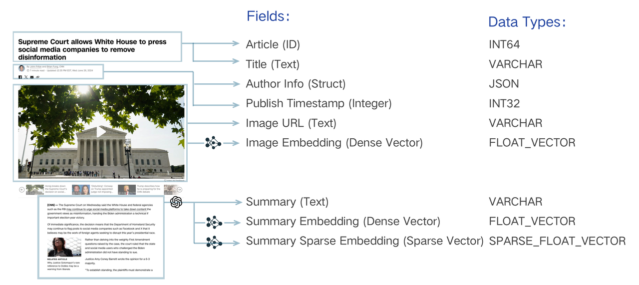
The data model design of a search system involves analyzing business needs and abstracting information into a schema-expressed data model. For instance, searching a piece of text must be "indexed" by converting the literal string into a vector through "embedding" and enabling vector search. Beyond this essential requirement, storing other properties such as publication timestamp and author may be necessary. This metadata allows for semantic searches to be refined through filtering, returning only texts published after a specific date or by a particular author. You can also retrieve these scalars with the main text to render the search result in the application. Each should be assigned a unique identifier to organize these text pieces, expressed as an integer or string. These elements are essential for achieving sophisticated search logic.
Refer to Schema Design Hands-On to figure out how to make a well-designed schema.
# Create Schema
The following code snippet demonstrates how to create a schema.
from pymilvus import MilvusClient, DataType

schema = MilvusClient.create_schema()
2
3
# Add Primary Field
The primary field in a collection uniquely identifies an entity. It only accepts Int64 or VarChar values. The following code snippets demonstrate how to add the primary field.
schema.add_field(
    field_name="my_id",
    "datatype=DataType.INT64",
    is_primary=True,
    auto_id=False,
)
2
3
4
5
6
When adding a field, you can explicitly clarify the field as the primary field by setting its is_primary property to True. A primary field accepts Int64 values by default. In this case, the primary field value should be integers similar to 12345. If you choose to use VarChar values in the primary field, the value should be strings similar to my_entity_1234.
You can also set the autoId properties to True to make Zilliz Cloud automatically allocate primary field values upon data insertions.
For details, refer to Primary Field & AutoId.
# Add Vector Fields
Vector fields accept various sparse and dense vector embeddings. On Zilliz Cloud, you can add four vector fields to a collection. The following code snippets demonstrate how to add a vector field.
schema.add_field(
    field_name="my_vector",
    datatype=DataType.FLOAT_VECTOR,
    dim=5
)
2
3
4
5
The dim parameter in the above code snippets indicates the dimensionality of the vector embeddings to be held in the vector field. The FLOAT_VECTOR value indicates that the vector field holds a list of 32-bit floating numbers, which are usually used to represent antilogarithms. In addition to that, Zilliz Cloud also supports the following types of vector embeddings:
FLOAT16_VECTOR: A vector field of this type holds a list of 16-bit half-precision floating numbers and usually applies to memory-or-bandwidth-restricted deep learning or GPU-based computing scenarios.BFLOAT16_VECTOR: A vector field of this type holds a list of 16-bit floating-point numbers that have reduced precision but the same exponent range as Float32. This type of data is commonly used in deep learning scenarios, as it reduces memory usage without significantly impacting accuracy.INT8_VECTOR: A vector field of this type stores vectors composed of 8-bit signed integers (int8), with each component ranging from -128 to 127. Tailored or quantized deep learning architectures -- such as ResNet and EfficientNet -- it substantially shrinks model size and boosts inference speed, all while incurring only minimal precision loss. Note: This vector type is supported only for HNSW indexes.BINARY_VECTOR: A vector field of this type holds a list of 0s and 1s. They serve as compact features for representing data in image processing and information retrieval scenarios.SPARSE_FLOAT_VECTOR: A vector field of this type holds a list of non-zero numbers and their sequence numbers to represent sparse vector embeddings.
# Add Scalar Fields
In common cases, you can use scalar fields to store the metadata of the vector embeddings stored in Milvus, and conduct ANN searches with metadata filtering to improve the correctness of the search results. Zilliz Cloud supports multiple scalar field types, including VarChar, Boolean, Int, Float, Double, Array, and JSON.
# Add String Fields
In Milvus, you can use VarChar fields to store strings. For more on the VarChar field, refer to String Field.
schema.add_field(
    field_name="my_varchar",
    datatype=DataType.VARCHAR,
    max_length=512
)
2
3
4
5
# Add Number Fields
The types of numbers that Milvus supports are Int8, Int16, Int32, Int64, Float, and Double. For more on the number fields, refer to Number Field.
schema.add_field(
    field_name="my_int64",
    datatype=DataType.INT64
)
2
3
4
# Add Boolean Fields
Milvus supports boolean fields. The following code snippets demonstrate how to add a boolean field.
schema.add_field(
    field_name="my_bool",
    datatype=DataType.BOOL,
)
2
3
4
# Add JSON fields
A JSON field usually stores half-structured JSON data. For more on the JSON fields, refer to JSON Field.
schema.add_field(
    field_name="my_json",
    datatype=DataType.JSON,
)
2
3
4
# Add Array Fields
An array field stores a list of elements. The data types of all elements in an array field should be the same. For more on the array fields, refer to Array Field.
schema.add_field(
    field_name="my_array",
    datatype=DataType.ARRAY,
    element_type=DataType.VARCHAR,
    max_capacity=5,
    max_length=512,
)
2
3
4
5
6
7
# Primary Field & AutoID
The primary field uniquely identifies an entity. This page introduces how to add the primary field of two different data types and how to enable Milvus to automatically allocate primary field values.
# Overview
In a collection, the primary key of each entity should be globally unique. When adding the primary field, you need to explicitly set its data type to VARCHAR or INT64. Setting its data type to INT64 indicates that the primary keys should be an integer similar to 12345; Setting its data type to VARCHAR indicates that the primary keys should be a string similar to my_entity_1234.
You can also enable AutoID to make Milvus automatically allocate primary keys for incoming entities. Once you have enabled AutoID in your collection, do not include primary keys when inserting entities.
The primary field in a collection does not have a default value and cannot be null.
NOTE
- A standard
insertoperation with a primary key that already exists in the collection will not overwrite the old entry. Instead, it will create a new, separate entity with the same primary key. This can lead to unexpected search results and data redundancy. - If your use case involves updating existing data or you suspect that the data you are inserting may already exist, it is highly recommended to use the upsert operation. The upsert operation will intelligently update the entity if the primary key exists, or insert a new one if it does not. For more details, refer to Upsert Entities.
# Use Int64 Primary Keys
To use primary keys of the Int64 type, you need to set datatype to DataType.INT64 and set is_primary to true. If you also need Milvus to allocate the primary keys for the incoming entities, also set auto_id to true.
from pymilvus import MilvusClient, DataType

schema = MilvusClient.create_schema()

schema.add_field(
    field_name="my_id",
    datatype=DataType.INT64,
    is_primary=True,
    auto_id=True,
)
2
3
4
5
6
7
8
9
10
# Use VarChar Primary Keys
To use VarChar primary keys, in addition to changing the value of the data_type parameter to DataType.VARCHAR, you also need to set the max_length parameter for the field.
schema.add_field(
    field_name="my_id",
    datatype=DataType.VARCHAR,
    is_primary=True,
    auto_id=True,
    max_length=512,
)
2
3
4
5
6
7
# Dense Vector
Dense vectors are numerical data representations widely used in machine learning and data analysis. The consist of arrays with real numbers, where most or all elements are non-zero. Compared to sparse vectors, dense vectors contain more information at the same dimensional level, as each dimonsion holds meaningful values. This representation can effectively capture complex patterns and relationships, making data easier to analyze and process in high-dimensional spaces. Dense vectors typically have a fixed number of dimensions, ranging from a few dozen to several hundred or even thousands, depending on the specific application and requirements.
Dense vectors are mainly used in scenarios that require understanding the semantics of data, such as semantic search and recommendation systems. In semantic search, dense vectors help capture the underlying connections between queries and documents, improving the relevance of search results. In recommendation systems, they aid in identifying similarities between users and items, offering more personalized suggestions.
# Overview
Dense vectors are typically represented as arrays of floating-point numbers with a fixed length, such as [0.2, 0.7, 0.1, 0.8, 0.3, ..., 0.5]. The dimensionality of these vectors usually ranges from hundreds to thousands, such as 128,256,768, or 1024. Each dimension captures specific semantic features of an object, making it applicable to various scenarios through similarity calculations.
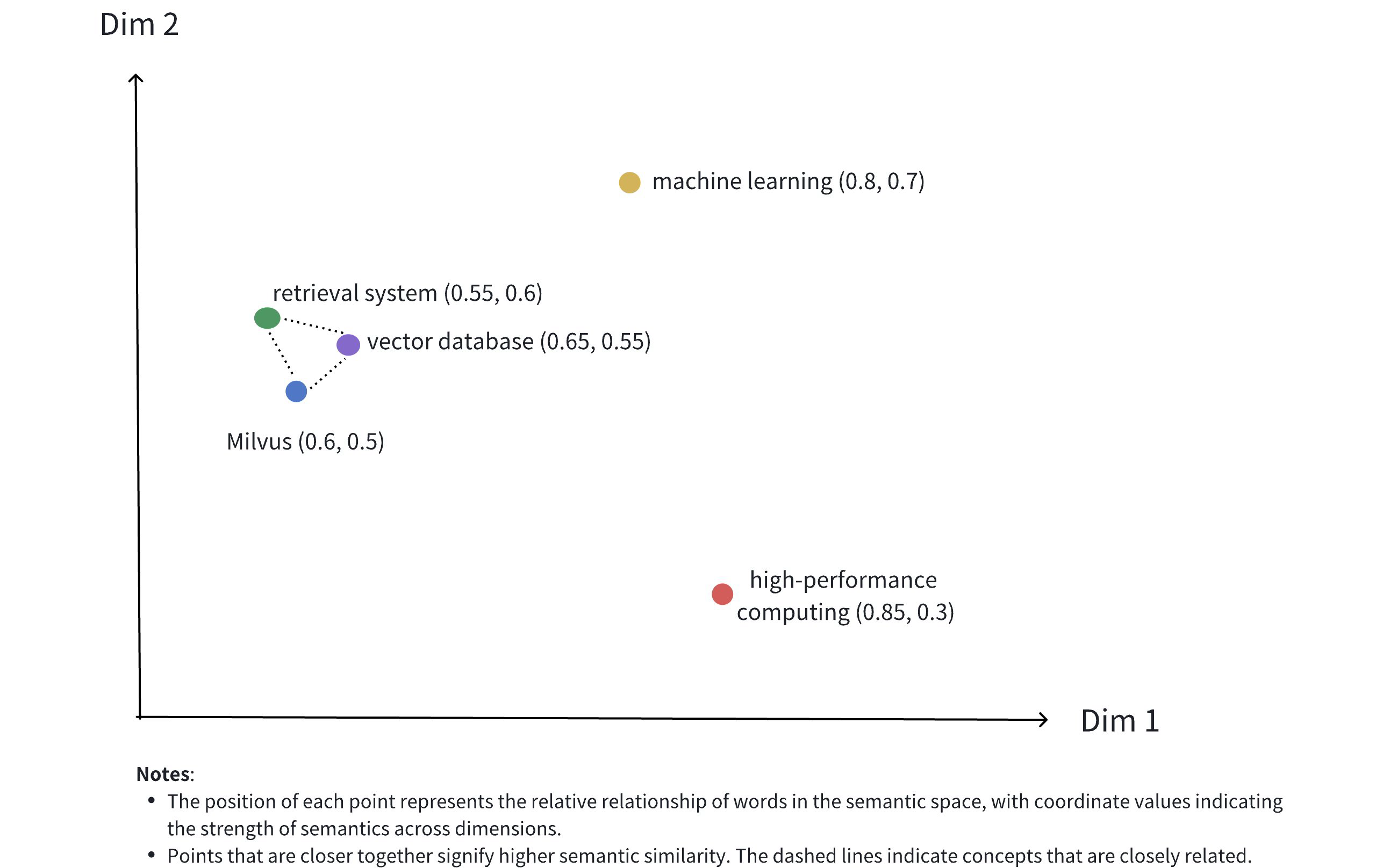
The image above illustrates the representation of dense vectors in a 2D space. Although dense vectors in real-world applications often have much higher dimensions, this 2D illustration effectively conveys serveral concepts:
- Multidimensional Representation: Each point represents a conceptual object (like Milvus, vector database, retrieval system, etc.), with its position determined by the values of its dimensions.
- Semantic Relationships: The distances between points reflect the semantic similarity between concepts. Closer points indicate concepts that are more semantically related.
- Clustering Effect: Related concepts (such as Milvus, vector database, and retrieval system) are positioned close to each other in space, forming a semantic cluster.
Below is an example of a real dense vector representing the text "Milvus is an efficient vector database":
[
    -0.013052909,
    0.020387933,
    -0.007869,
    -0.11111383,
    -0.030188112,
    -0.0053388323,
    0.0010654867,
    0.072027855,
    # ... more dimensions
]
2
3
4
5
6
7
8
9
10
11
Dense vectors can be generated using various embedding models, such as CNN models (like ResNet, VGG) for images and language models (like BERT, Word2Vec) for text. These models transform raw data into points in high-dimensional space, capturing the semantic features of the data. Additionally, Milvus offers convenient methods to help users generate and process dense vectors, as detailed in Embeddings.
Once data is vectorized, it can be stored in Milvus for management and vector retrieval. The diagram below shows the basic process.

NOTE
Besides dense vectors, Milvus also supports sparse vectors and binary vectors. Sparse vectors are suitable for precise matches based on specific terms, such as keyword search and term matching, while binary vectors are commonly used for efficiently handling binarized data, such as image pattern matching and certain hashing applications. For more information, refer to Binary Vector and Sparse Vector.
# Use dense vectors
# Add vector field
To use dense vectors in Milvus, first define a vector field for storing dense vectors when creating a collection. This process includes:
- Setting
datatypeto a supported dense vector data type. For supported dense vector data types, see Data Types. - Specifying the dimensions of dense vector using the
dimparameter.
In the example below, we add a vector field named dense_vector to store dense vectors. The field's data type is FLOAT_VECTOR, with a demension of 4.
from pymilvus import MilvusClient, DataType

client = MilvusClient(uri="http://localhost:19530")

schema = client.create_schema(
    auto_id=True,
    enable_dynamic_fields=True,
)

schema.add_field(field_name="pk", datatype=DataType.VARCHAR, is_primary=True, max_length=100)
schema.add_field(field_name="dense_vector", datatype=DataType.FLOAT_VECTOR, dim=4)
2
3
4
5
6
7
8
9
10
11
Supported data types for dense vector fields:
| Data Type | Description |
|---|---|
FLOAT_VECTOR | Stores 32-bit floating-point numbers, commonly used for representing real numbers in scientific computations and machine learning. Ideal for scenarios requiring high precision, such as distinguishing similar vectors. |
FLOAT16_VECTOR | Stores 16-bit half-precision floating-point numbers, used for deep learning and GPU computations. It saves storage space in scenarios where precision is less critical, such as in the low-precision recall phase of recommendation systems. |
BFLOAT_16_VECTOR | Stores 16-bit Brain Floating Point (bfloat16) numbers, offering the same range of exponents as Float32 but with reduced precision. Suitable for scenarios that need to process large volumes of vectors quickly, such as large-scale image retrieval. |
INT8_VECTOR | Stores vectors whose individual elements in each dimension are 8-bit integers (int8), with each element ranging from -128 to 127. Designed for quantized deep learning models (e.g., ResNet, EfficientNet), INT8_VECTOR reduces model size and speeds up inference with minimal precision loss. Note: This vector type is supported only for HNSW indexes. |
# Set index params for vector field
To accelerate semantic searches, an index must be created for the vector field. Indexing can significantly improve the retrieval efficiency of large-scale data.
index_params = client.prepare_index_params()

index_params.add_index(
    field_name="dense_vector",
    index_name="dense_vector_index",
    index_type="AUTOINDEX",
    metric_type="IP"
)
2
3
4
5
6
7
8
In the example above, an index named dense_vector_index is created for the dense_vector field using the AUTOINDEX index type. The metric_type is set to IP, indicating that inner product will be used as the distance metric.
Milvus provides various index types for a better vector search experience. AUTOINDEX is a special index type designed to smooth the learning curve of vector search. There are a lot of index types available for you to choose from.
Milvus supports other metric types. For more information, refer to Metric Types.
# Create collection
Once the dense vector and index param settings are complete, you can create a collection containing dense vectors. The example below uses the create_collection method to create a collection named my_collection.
client.create_collection(
    collection_name="my_collection",
    schema=schema,
    index_params=index_params
)
2
3
4
5
# Insert data
After creating the collection, use the insert method to add data containing dense vectors. Ensure that the dimensionality of the dense vectors being inserted matches the dim value defined when adding the dense vector field.
data = [
    {"dense_vector": [0.1, 0.2, 0.3, 0.7]},
    {"dense_vector": [0.2, 0.3, 0.4, 0.8]},
]

client.insert(
    collection_name="my_collection",
    data=data
)
2
3
4
5
6
7
8
9
# Perform similarity search
Semantic search based on dense vectors is one of the core features of Milvus, allowing you to quickly find data that is most similar to a query vector based on the distance between vectors. To perform a similarity search, prepare the query vector and search parameters, then call the search method.
search_params = {
    "params": {"nprobe": 10}
}

query_vector = [0.1, 0.2, 0.3, 0.7]

res = client.search(
    collection_name="my_collection",
    data=[query_vector],
    anns_field="dense_vector",
    search_params=search_params,
    limit=5,
    output_field=["pk"]
)

print(res)

# Output
# data: [
#     "[
#         {
#             'id': '453718927992172271',
#             'distance': 0.7599999904632568,
#             'entity': {'pk': '453718927992172271'}
#         },
#         {
#             'id': '453718927992172270',
#             'distance': 0.6299999952316284,
#             'entity': {'pk': '453718927992172270'}
#         }
#     ]"
# ]
2
3
4
5
6
7
8
9
10
11
12
13
14
15
16
17
18
19
20
21
22
23
24
25
26
27
28
29
30
31
32
For more information on similarity search parameters, refer to Basic ANN Search.
# Binary Vector
Binary vectors are a special form of data representation that convert traditional high-dimensional floating-point vectors into binary vectors containing only 0s and 1s. This transformation not only compresses the size of the vector but also reduces storage and computational costs while retaining semantic information. When precision for non-critical features is not essential, binary vectors can effectively maintain most of the integrity and utility of the original floating-point vectors.
Binary vectors have a wide range of applications, particularly in situations where computational efficiency and storage optimization are crucial. In large-scale AI systems, such as search engines or recommendation systems, real-time processing of massive amounts of data is key. By reducing the size of the vectors, binary vectors help lower latency and computational costs without significantly sacrificing accuracy. Additional, binary vectors are usefual in resource constrained environments, such as mobile devices and embedded systems, where memory and processing power are limited. Through the use of binary vectors, complex AI functions can be implemented in these restricted settings while maintaining high performance.
# Overview
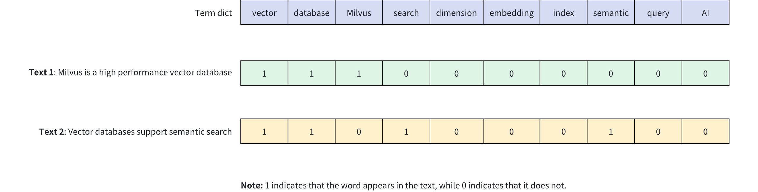
Binary vectors are a method of encoding complex objects (like images, text, or audio) into fixed-length binary values. In Milvus, binary vectors are typically represented as bit arrays or byte arrays. For example, an 8-dimensional binary vector can be represented as [1, 0, 1, 1, 0, 0, 1, 0].
The diagram below shows how binary vectors represent the presence of keywords in text content. In this example, a 10-dimensional binary vector is used to represent two different texts (Text 1 and Text 2), where each dimension corresponds to a word in the vocabulary: 1 indicates the presence of the word in the text, while 0 indicates its absence.
Binary vectors have the following characteristics:
- Efficient Storage: Each dimension requires only 1 bit of storage, significantly reducing storage space.
- Fast Computation: Similarity between vectors can be quickly calculated using bitwise operations like XOR.
- Fixed Length: The length of the vector remains constant regardless of the original text length, making indexing and retrieval easier.
- Simple and Intuitive: Directly reflects the presence of keywords, making it suitable for certain specialized retrieval tasks.
Binary vectors can be generated through various methods. In text processing, predefined vocabularies can be used to set corresponding bits based on word presence. For image processing, perceptual hashing algorithms (like pHash) can generate binary features of images. In machine learning applications, model outputs can be binarized to obtain binary vector representations.
After binary vectorization, the data can be stored in Milvus for management and vector retrieval. The diagram below shows the basic process.

NOTE
Although binary vectors excel in specific scenarios, they have limitations in their expressive capability, making it difficult to capture complex semantic relationships. Therefore, in real-world scenarios, binary vectors are often used alongside other vector types to balance efficiency and expressiveness. For more information, refer to Dense Vector and Sparse Vector.
# Use binary vectors
# Add vector field
To use binary vectors in Milvus, first define a vector field for storing binary vectors when creating a collection. This process includes:
- Setting
datatypeto the supported binary vector data type, i.e.,BINARY_VECTOR. - Specifying the vector's dimensions using the
dimparameter. Note thatdimmust be a multiple of 8 as binary vectors must be converted into a byte array when inserting. Every 8 boolean values (0 or 1) will be packed into 1 byte. For example, ifdim=128, a 16-byte arra is required for insertion.
from pymilvus import MilvusClient, DataType

client = MilvusClient(uri="http://localhost:19530")

schema = client.create_schema(
    auto_id=True,
    enable_dynamic_fields=True,
)

schema.add_field(field_name="pk", datatype=DataType.VARCHAR, is_primary=True, max_length=100)
schema.add_field(field_name="binary_vector", datatype=DataType.BINARY_VECTOR, dim=128)
2
3
4
5
6
7
8
9
10
11
In this example, a vector field named binary_vector is added for storing binary vectors. The data type of this field is BINARY_VECTOR, with a dimension of 128.
# Set index params for vector field
To Speed up searches, an index must be created for the binary vector field. Indexing can significantly enhance the retrieval efficiency of large-scale vector data.
index_params = client.prepare_index_params()

index_params.add_index(
    field_name="binary_vector",
    index_name="binary_vector_index",
    index_type="AUTOINDEX",
    metric_type="HAMMING"
)
2
3
4
5
6
7
8
In the example above, an index named binary_vector_index is created for the binary_vector field, using the AUTOINDEX index type. The metric_type is set to HAMMING, indicating that Hamming distance is used for similarity measurement.
Milvus provides various index types for a better vector search experience. AUTOINDEX is a special index type designed to smooth the learning curve of vector search. There are a lot of index types available for you to choose from. For details, refer to Index Explained.
Additionally, Milvus supports other similarity metrics for binary vectors. For more information, refer to Metric Types.
# Create collection
Once the binary vector and index settings are complete, create a collection that contains binary vectors. The example below uses the create_collection method to create a collection named my_collection.
client.create_collection(
    collection_name="my_collection",
    schema=schema,
    index_params=index_params
)
2
3
4
5
# Insert data
After creating the collection, use the insert method to add data containing binary vectors. Note that binary vectors should be provided in the form of a byte array, where each byte represents 8 boolean values.
For example, for a 128-dimensional binary vector, a 16-byte array is required (since 128 bits ÷ 8 bits/byte = 16 bytes). Below is an example code for inserting data:
def convert_bool_list_to_bytes(bool_list):
    if len(bool_list) % 8 != 0:
        raise ValueError("The length of a boolean list must be a multiple of 8")

    byte_array = bytearray(len(bool_list) // 8)
    for i, bit in enumerate(bool_list):
        if bit == 1:
            index = i // 8
            shift = i % 8
            byte_array[index] |= (1 << shift)
    return bytes(byte_array)

bool_vectors = [
    [1, 0, 0, 1, 1, 0, 1, 1, 0, 1, 0, 1, 0, 1, 0, 0] + [0] * 112,
    [0, 1, 0, 1, 0, 1, 0, 0, 1, 1, 0, 0, 1, 1, 0, 1] + [0] * 112,
]

data = [{"binary_vector": convert_bool_list_to_bytes(bool_vector) for bool_vector in bool_vectors}]

client.insert(
    collection_name="my_collection",
    data=data
)
2
3
4
5
6
7
8
9
10
11
12
13
14
15
16
17
18
19
20
21
22
23
# Perform similarity search
Similarity search is one of the core features of Milvus, allowing you to quickly find data that is most similar to a query vector based on the distance between vectors. To perform a similarity search using binary vectors, prepare the query vector and search parameters, the call the search method.
During search operations, binary vectors must also be provided in the form of a byte array. Ensure that the dimensionality of the query vector matches the dimension specified when defining dim and that every 8 boolean values are converted into 1 byte.
search_params = {
    "params": {"nprobe": 10}
}

query_bool_list = [1, 0, 0, 1, 1, 0, 1, 1, 0, 1, 0, 1, 0, 1, 0, 0] + [0] * 112
query_vector = convert_bool_list_to_bytes(query_bool_list)

res = client.search(
    collection_name="my_collection",
    data=[query_vector],
    anns_field="binary_vector",
    search_params=search_params,
    limit=5,
    output_fields=["pk"]
)

print(res)

# Output
# data: ["[{'id': '453718927992172268', 'distance': 10.0, 'entity': {'pk': '453718927992172268'}}]"]
2
3
4
5
6
7
8
9
10
11
12
13
14
15
16
17
18
19
20
For more information on similarity search parameters, refer to Basic ANN Search.
# Sparse Vector
Sparse vectors are an important method of capturing surface-level term matching in information retrieval and natural language processing. While dense vectors excel in semantic understanding, sparse vectors often provide more predictable matching results, especially when searching for special terms or textual identifiers.
# Overview
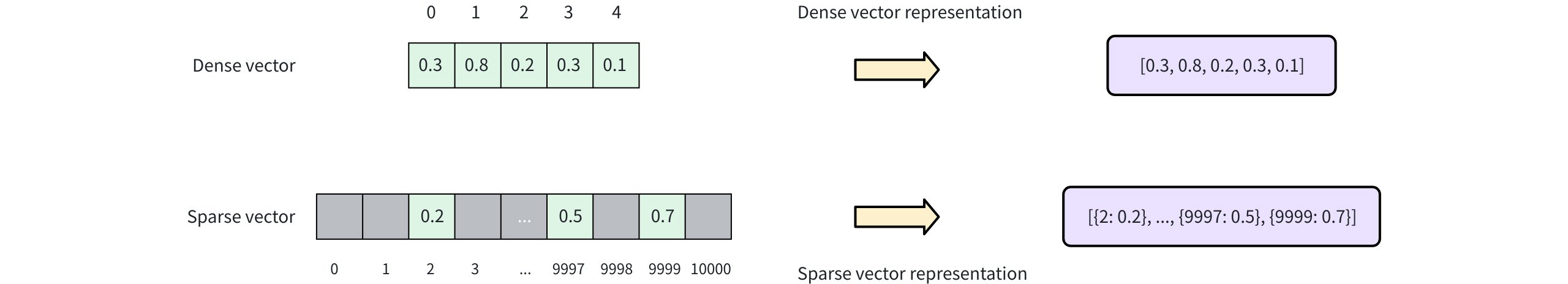
A sparse vector is a special high-dimensional vector where most elements are zero, and only a few dimensions have non-zero values. As shown in the diagram below, dense vectors are typically represented as continuous arrays where each position has a value (e.g., [0.3, 0.8, 0.2, 0.3, 0.1]). In contrast, sparse vectors store only non-zero elements and their indices of the dimension, often represented as key-value pairs of { index: value } (e.g., [{2: 0.2}, ..., {9997: 0.5}, {9999: 0.7}]).
With tokenization and scoring, documents can be represented as bag-of-words vectors, where each dimension corresponds to a specific word in the vocabulary. Only the words present in the document have non-zero values, creating a sparse vector representation. Sparse vectors can be generated using two approaches:
- Traditional statistical techniques: such as TF-IDF(Term Frequency-Inverse Document Frequency) and BM25(Best Matching 25), assign weights to words based on their frequency and importance across a corpus. These methods compute simple statistics as scores for each dimension, which represents a token. Milvus provides built-in full-text search with the BM25 method, which automatically converts text into sparse vectors, eliminating the need for manual preprocessing. This approach is ideal for keyword-based search, where precision and exact matches are important. Refer to Full Text Search for more information.
- Neural sparse embedding models: are learned methods to generate sparse representations by training on large datasets. They are typically deep learning models with Transformer architecture, able to expand and weigh terms based on semantic context. Milvus also supports externally generated sparse embeddings from models like SPLADE. See Embeddings for details.
Sparse vectors and the original text can be stored in Milvus for efficient retrieval. The diagram below outlines the overall process.

NOTE
In addition to sparse vectors, Milvus also supports dense vectors and binary vectors. Dense vectors are ideal for capturing deep semantic relationships, while binary vectors excel in scenarios like quick similarity comparisions and content deduplication. For more information, refer to Dense Vector and Binary Vector.
# Data Formats
In the following sections, we demonstrate how to store vectors from learned sparse embedding models like SPLADE. If you are looking form something to complement dense-vector-based semantic search, we recommend Full Text Search with BM25 over SPLADE for simplicity. If you're ran quality evaluation and dediced to use SPLADE, you can refer to Embeddings on how to generate sparse vectors with SPLADE.
Milvus supports sparse vector input with the following formats:
- List of Dictionaries (formatted as
{dimension_index: value, ...})
# Represent each sparse vector using a dictionary
sparse_vectors = [{27: 0.5, 100: 0.3, 5369: 0.6} , {100: 0.1, 3: 0.8}]
2
- Sparse Matrix (using the
scipy.sparseclass)
from scipy.sparse import csr_matrix

# First vector: indices [27, 100, 5369] with values [0.5, 0.3, 0.6]
# Second vector: indices [3, 100] with values [0.8, 0.1]
indices = [[27, 100, 5369], [3, 100]]
values = [[0.5, 0.3, 0.6], [0.8, 0.1]]
sparse_vectors = [csr_matrix((vals, ([0]*len(idx), idx)), shape=(1, 5369+1)) for idx, vals in zip(indices, values)]
2
3
4
5
6
7
- List of Tuple Iterables (e.g.
[(dimension_index, value)])
# Represent each sparse vector using a list of iterables (e.g. tuples)
sparse_vector = [
    [(27, 0.5), (100, 0.3), (5369, 0.6)],
    [(100, 0.1), (3, 0.8)]
    ]
2
3
4
5
# Define Collection Schema
Before creating a collection, you need to specify the collection schema, which defines fields and optionally a function to convert a text field into corresponding sparse vector representation.
# Add fields
To use sparse vectors in Milvus, you need to create a collection with a schema including the following fields:
- A
SPARSE_FLOAT_VECTORfield reserved for storing sparse vectors, either auto-generated from aVARCHARfield or provided directly in the input data. - Typically, the raw text that the sparse vector represents is also stored in the collection. You can use a
VARCHARfield for storing the raw text.
from pymilvus import MilvusClient, DataType

client = MilvusClient(uri="http://localhost:19530")

schema = client.create_schema(
    auto_id=True,
    enable_dynamic_fields=True,
)

schema.add_field(field_name="pk", datatype="DataType.VARCHAR", is_primary=True, max_length=100)
schema.add_field(field_name="sparse_vector", datatype=DataType.SPARSE_FLOAT_VECTOR)
schema.add_field(field_name="text", datatype=DataType.VARCHAR, max_length=65535, enable_analyzer=True)
2
3
4
5
6
7
8
9
10
11
12
In this example, three fields are added:
pk: This field stores primary keys using theVARCHARdata type, which is auto-generated with a maximum length of 100 bytes.sparse_vector: This field stores sparse vectors using theSPARSE_FLOAT_VECTORdata type.text: This field stores text strings using theVARCHARdata type, with a maximum length of 65535 bytes.
NOTE
To enable Milvus or to generate sparse vector embeddings from a specified text field during data insertion, an additional step involving a function must be taken. For more information, please refer to Full Text Search.
# Set Index Parameters
The process of creating an index for sparse vectors is similar to that for dense vectors, but with differences in the specified index type (index_type), distance metric (metric_type), and index parameters (params).
index_params = client.prepare_index_params()

index_params.add_index(
    field_name="sparse_vector",
    index_name="sparse_inverted_index",
    index_type="SPARSE_INVERTED_INDEX",
    metric_type="IP",
    params={"inverted_index_algo": "DAAT_MAXSCORE"}, # or "DAAT_WAND" or "TAAT_NAIVE"
)
2
3
4
5
6
7
8
9
This example uses the SPARSE_INVERTED_INDEX index type with IP as the metric. For more details, see the following resources:
- SPARSE_INVERTED_INDEX: Explained index and its parameters.
- Metric Types: Supported metric types for different field types.
- Full Text Search: A detailed tutorial on full-text search.
# Create Collection
Once the sparse vector and index settings are complete, you can create a collection that contains sparse vectors. The example below uses the create_collection method to create a collection named my_collection.
client.create_collection(
    collection_name="my_collection",
    schema=schema,
    index_params=index_params
)
2
3
4
5
# Insert Data
You must provide data for all fields defined during collection creation, except for fields that are auto-generated (such as the primary key with auto_id enabled). If you are using the build-in BM25 function to auto-generate sparse vectors, you should also omit the sparse vector field when inserting data.
data = [
    {
        "text": "information retrieval is a field of study.",
        "sparse_vector": {1: 0.5, 100: 0.3, 500: 0.8}
    },
    {
        "text": "information retrieval focuses on finding relevant information in large datasets.",
        "sparse_vector": {10: 0.1, 200: 0.7, 1000: 0.9}
    }
]

client.insert(
    collection_name="my_collection",
    data=data
)
2
3
4
5
6
7
8
9
10
11
12
13
14
15
# Perform Similarity Search
To perform a similarity search using sparse vectors, prepare both the query data and the search parameters.
# Prepare search parameters
search_params = {
    "params": {"drop_ratio_search": 0.2}, # A tunable drop ratio parameter with a valid range between 0 and 1
}

# Query with sparse vector
query_data = [{1: 0.2, 50: 0.4, 1000: 0.7}]
2
3
4
5
6
7
Then, execute the similarity search using the search method:
res = client.search(
    collection_name="my_collection",
    data=query_data,
    limit=3,
    output_fields=["pk"],
    search_params=search_params,
    consistency_level="Strong"
)

print(res)

# Output
#
# data:
#[
  #"[
    #{
      #'id': '453718927992172266',
      #'distance': 0.6299999952316284,
      #'entity': {'pk': '453718927992172266'}},
    #{
      #'id': '453718927992172265',
      #'distance': 0.10000000149011612,
      #'entity': {'pk': '453718927992172265'}
    #}
  #]"
#]
2
3
4
5
6
7
8
9
10
11
12
13
14
15
16
17
18
19
20
21
22
23
24
25
26
27
# String Field
In Milvus, VARCHAR is the data type used for storing string data. When you define a VARCHAR field, two parameters are mandatory:
- Set the
datatypetoDataType.VARCHAR. - Specify the
max_length, which defines the maximum number of bytes theVARCHARfield can store. The valid range formax_lengthis from 1 to 65535.
NOTE
Milvus supports null values and default values for VARCHAR fields. To enable these features, set nullable to True and default_value to a string value. For details, refer to Nullable & Default.
# Add VARCHAR field
To store string data in Milvus, define a VARCHAR field in your collection schema. Below is an example of defining a collection schema with two VARCHAR fields:
varchar_field1: stores up to 100 bytes, allows null values, and has a default value of"Unkown".varchar_field2: stores up to 200 bytes, allows null values, but does not have a default value.
NOTE
If you set enable_dynamic_fields=True when defining the schema, Milvus allows you to insert scalar fields that were not defined in advance. However, this may increase the complexity of queries and management, potentially impacting performance. For more information, refer to Dynamic Field.
# Import necessary libraries
from pymilvus import MilvusClient, DataType

# Define server address
SERVER_ADDR = "http://localhost:19530"

# Create a MilvusClient instance
client = MilvusClient(uri=SERVER_ADDR)

# Define the collection schema
schema = client.create_schema(
    auto_id=False,
    enable_dynamic_field=True,
)

# Add `varchar_field1` that supports null values with default value "Unkown"
schema.add_field(field_name="varchar_field1", datatype=DataType.VARCHAR, max_length=100, nullable=True, default_value="Unkown")
# Add `varchar_field2` that supports null values without default value
schema.add_field(field_name="varchar_field2", datatype=DataType.VARCHAR, max_length=200, nullable=True)
schema.add_field(field_name="pk", datatype=DataType.INT64, is_primary=True)
schema.add_field(field_name="embedding", datatype=DataType.FLOAT_VECTOR, dim=3)
2
3
4
5
6
7
8
9
10
11
12
13
14
15
16
17
18
19
20
21
# Set index params
Indexing helps improve search and query performance. In Milvus, indexing is mandatory for vector fields but optional for scalar fields.
The following example creates indexes on the vector field embedding and the scalar field varchar_field1, both using the AUTOINDEX index type. With this type, Milvus automatically selects the most suitable index based on the data type. You can also customize the index type and params for each field. For details, refer to Index Explained.
# Set index params
index_params = client.prepare_index_params()

# Index `varchar_field1` with AUTOINDEX
index_params.add_index(
    field_name="varchar_field1",
    index_type="AUTOINDEX",
    index_name="varchar_index"
)

# Index `embedding` with AUTOINDEX and specify metric_type
index_params.add_index(
    field_name="embedding",
    index_type="AUTOINDEX", # Use automatic indexing to simplify complex index settings
    index_name="COSINE" # Specify similarity metric type, options include L2, COSINE, or IP
)
2
3
4
5
6
7
8
9
10
11
12
13
14
15
16
# Create collection
Once the schema and index are defined, create a collection that includes string fields.
# Create Collection
client.create_collection(
    collection_name="my_collection",
    schema=schema,
    index_params=index_params
)
2
3
4
5
6
# Insert data
After creating the collection, insert entities that match the schema.
# Sample data
data = [
    {"varchar_field1": "Product A", "varchar_field2": "High quality product", "pk": 1, "embedding": [0.1, 0.2, 0.3]},
    # varchar_field2 field is missing, which should be NULL
    {"varchar_field1": "Product B", "pk": 2, "embedding": [0.4, 0.5, 0.6]},
    # `varchar_field1` should default to `Unknown`, `varchar_field2` is NULL
    {"varchar_field1": None, "varchar_field2": None, "pk": 3, "embedding": [0.2, 0.3, 0.1]},
    # `varchar_field2` is NULL
    {"varchar_field1": "Product C", "varchar_field2": None, "pk": 4, "embedding": [0.5, 0.7, 0.2]},
    # `varchar_field1` should default to `Unknown`
    {"varchar_field1": None, "varchar_field2": "Exclusive deal", "pk": 5, "embedding": [0.6, 0.4, 0.8]},
    # `varchar_field2` is NULL
    {"varchar_field1": "Unknown", "varchar_field2": None, "pk": 6, "embedding": [0.8, 0.5, 0.3]},
    # Empty string is not treated as NULL
    {"varchar_field1": "", "varchar_field2": "Best seller", "pk": 7, "embedding": [0.8, 0.5, 0.3]},
]

# Insert data
client.insert(
    collection_name="my_collection",
    data=data
)
2
3
4
5
6
7
8
9
10
11
12
13
14
15
16
17
18
19
20
21
22
# Query with filter expressions
After inserting entities, use the query method to retrieve entites that match the specified filter expressions.
To retrieve entities where the varchar_field1 matches the string "Product A":
# Filter `varchar_field1` with value "Product A"
filter = 'varchar_field1 == "Product A"'

res = client.query(
    collection_name="my_collection",
    filter=filter,
    output_fields=["varchar_field1", "varchar_field2"]
)

print(res)

# Example output:
# data: [
#     "{'varchar_field1': 'Product A', 'varchar_field2': 'High quality product', 'pk': 1}"
# ]
2
3
4
5
6
7
8
9
10
11
12
13
14
15
To retrieve entities where the varchar_field2 is null:
# Filter entities where `varchar_field2` is null
filter = 'varchar_field2 is null'

res = client.query(
    collection_name="my_collection",
    filter=filter,
    output_fields=["varchar_field1", "varchar_field2"]
)

print(res)

# Example output:
# data: [
#     "{'varchar_field1': 'Product B', 'varchar_field2': None, 'pk': 2}",
#     "{'varchar_field1': 'Unknown', 'varchar_field2': None, 'pk': 3}",
#     "{'varchar_field1': 'Product C', 'varchar_field2': None, 'pk': 4}",
#     "{'varchar_field1': 'Unknown', 'varchar_field2': None, 'pk': 6}"
# ]
2
3
4
5
6
7
8
9
10
11
12
13
14
15
16
17
18
To retrieve entities where varchar_field1 has the value "Unkown", use the following expression below. As the default value of varchar_field1 is "Unkown", the expected result should include entities with varchar_field1 explicitly set to "Unkown" or with varchar_field1 set to null.
# Filter entities with `varchar_field1` with value `Unkown`
filter = 'varchar_field1 == "Unkown"'

res = client.query(
    collection_name="my_collection",
    filter=filter,
    output_fields=["varchar_field1", "varchar_field2"]
)

print(res)

# Example output:
# data: [
#     "{'varchar_field1': 'Unknown', 'varchar_field2': None, 'pk': 3}",
#     "{'varchar_field1': 'Unknown', 'varchar_field2': 'Exclusive deal', 'pk': 5}",
#     "{'varchar_field1': 'Unknown', 'varchar_field2': None, 'pk': 6}"
# ]
2
3
4
5
6
7
8
9
10
11
12
13
14
15
16
17
# Vector search with filter expressions
In addition to basic scalar field filtering, you can combine vector similarity searches with scalar field filters. For example, the following code shows how to add a scalar field filter to a vector search:
# Search with string filtering

# Filter `varchar_field2` with value "Best seller"
filter = 'varchar_field2 == "Best seller"'

res = client.search(
    collection_name="my_collection",
    data=[[0.3, -0.6, 0.1]],
    limit=5,
    search_params={"params": {"nprobe": 10}},
    output_fields=["varchar_field1", "varchar_field2"],
    filter=filter
)

print(res)

# Example output:
# data: [
#     "[{'id': 7, 'distance': -0.04468163847923279, 'entity': {'varchar_field1': '', 'varchar_field2': 'Best seller'}}]"
# ]
2
3
4
5
6
7
8
9
10
11
12
13
14
15
16
17
18
19
20
# Number Field
A number field is a scalar field that stores numeric values. These values can be whole numbers (integer) or decimal numbers (floating-point numbers). They are typically used to represent quantities, measurements, or any data that needs to be mathematically processed.
The table below describes the data types of number fields available in Milvus.
| Field Type | Description |
|---|---|
BOOL | Boolean type for storing true or false, suitable for describing binary states. |
INT8 | 8-bit integer, suitable for storing small-range integer data. |
INT16 | 16-bit integer, for medium-range integer data. |
INT32 | 32-bit integer, ideal for general integer data storage like product quantities or user IDs. |
INT64 | 64-bit integer, suitable for storing large-range data like timestamps or identifiers. |
FLOAT | 32-bit floating-point number, for data requiring general precision, such as ratings or temperature. |
DOUBLE | 64-bit double-precision floating-point number, for high-precision data like financial information or scientific calculations. |
To declare a number field, simply set the datatype to one of the available numeric data types. For example, DataType.INT64 for an integer field or DataType.FLOAT for a floating-point field.
NOTE
Milvus supports null values and default values for number fields. To enable these features, set nullable to True and default_value to a numeric value. For details, refer to Nullable & Default.
# Add number field
To store numeric data, define a number field in your collection schema. Below is an example of a collection schema with two number fields:
age: stores integer data, allows null values, and has a default value of18.price: stores float data, allows null values, but does not have a default value.
# Import necessary libraries
from pymilvus import MilvusClient, DataType

# Define server address
SERVER_ADDR = "http://localhost:19530"

# Create a MilvusClient instance
client = MilvusClient(uri=SERVER_ADDR)

# Define the collection schema
schema = client.create_schema(
    auto_id=False,
    enable_dynamic_fields=True,
)

# Add an INT64 field `age` that supports null values with default value 18
schema.add_field(field_name="age", datatype=DataType.INT64, nullable=True, default_value=18)
# Add a FLOAT field `price` that supports null values without default value
schema.add_field(field_name="price", datatype=DataType.FLOAT, nullable=True)
schema.add_field(field_name="pk", datatype=DataType.INT64, is_primary=True)
schema.add_field(field_name="embedding", datatype=DataType.FLOAT_VECTOR, dim=3)
2
3
4
5
6
7
8
9
10
11
12
13
14
15
16
17
18
19
20
21
# Set index params
Indexing helps improve search and query performance. In Milvus, indexing is mandatory for vector fields but optional for scalar fields.
The following example creates indexes on the vector field embedding and the scalar field age, both using the AUTOINDEX index type. With this type, Milvus automatically selects the most suitable index based on the data type. You can also customize the index type and params for each field. For details, refer to Index Explained.
# Set index params
index_params = client.prepare_index_params()

# Index `age` with AUTOINDEX
index_params.add_index(
    field_name="age",
    index_type="AUTOINDEX",
    index_name="age_index"
)

# Index `embedding` with AUTOINDEX and specify similarity metric type
index_params.add_index(
    field_name="embedding",
    index_type="AUTOINDEX", # Use automatic indexing to simplify complex index settings
    metric_type="COSINE" # Specify similarity metric type, options include L2, COSINE, or IP
)
2
3
4
5
6
7
8
9
10
11
12
13
14
15
16
# Create collection
Once the schema and indexes are defined, create a collection that includes number fields.
# Create Collection
client.create_collection(
    collection_name="my_collection",
    schema=schema,
    index_params=index_params
)
2
3
4
5
6
# Insert data
After creating the collection, insert entities that match the schema.
data = [
    {"age": 25, "price": 99.99, "pk": 1, "embedding": [0.1, 0.2, 0.3]},
    {"age": 30, "pk": 2, "embedding": [0.4, 0.5, 0.6]}, # `price` field is missing, which should be null
    {"age": None, "price": None, "pk": 3, "embedding": [0.2, 0.3, 0.1]},  # `age` should default to 18, `price` is null
    {"age": 45, "price": None, "pk": 4, "embedding": [0.9, 0.1, 0.4]},  # `price` is null
    {"age": None, "price": 59.99, "pk": 5, "embedding": [0.8, 0.5, 0.3]},  # `age` should default to 18
    {"age": 60, "price": None, "pk": 6, "embedding": [0.1, 0.6, 0.9]}  # `price` is null
]

client.insert(
    collection_name="my_collection",
    data=data
)
2
3
4
5
6
7
8
9
10
11
12
13
# Query with filter expressions
After inserting entities, use the query method to retrieve entities that match the specified filter expressions.
To retrieve entities where the age is greater than 30:
filter = 'age > 30'

res = client.query(
    collection_name="my_collection",
    filter=filter,
    output_fields=["age", "price", "pk"]
)

print(res)

# Example output:
# data: [
#     "{'age': 45, 'price': None, 'pk': 4}",
#     "{'age': 60, 'price': None, 'pk': 6}"
# ]
2
3
4
5
6
7
8
9
10
11
12
13
14
15
To retrieve entities where the price is null:
filter = 'price is null'

res = client.query(
    collection_name="my_collection",
    filter=filter,
    output_fields=["age", "price", "pk"]
)

print(res)

# Example output:
# data: [
#     "{'age': 30, 'price': None, 'pk': 2}",
#     "{'age': 18, 'price': None, 'pk': 3}",
#     "{'age': 45, 'price': None, 'pk': 4}",
#     "{'age': 60, 'price': None, 'pk': 6}"
# ]
2
3
4
5
6
7
8
9
10
11
12
13
14
15
16
17
To retrieve entities where age has the value 18, use the following expression below. As the default value of age is 18, the expected result should include entities with age explicitly set to 18 or with age set to null.
filter = 'age == 18'

res = client.query(
    collection_name="my_collection",
    filter=filter,
    output_fields=["age", "price", "pk"]
)

print(res)

# Example output:
# data: [
#     "{'age': 18, 'price': None, 'pk': 3}",
#     "{'age': 18, 'price': 59.99, 'pk': 5}"
# ]
2
3
4
5
6
7
8
9
10
11
12
13
14
15
# Vector search with filter expressions
In addition to basic number field filtering, you can combine vector similarity searches with number field filters. For example, the following code shows how to add a number field filter to a vector search:
filter = "25 <= age <= 35"

res = client.search(
    collection_name="my_collection",
    data=[[0.3, -0.6, 0.1]],
    limit=5,
    search_params={"params": {"nprobe": 10}},
    output_fields=["age", "price"],
    filter=filter
)

print(res)

# Example output:
# data: [
#     "[{'id': 2, 'distance': -0.2016308456659317, 'entity': {'age': 30, 'price': None}},
#     {'id': 1, 'distance': -0.23643313348293304, 'entity': {'age': 25, 'price': 99.98999786376953}}]"
# ]
2
3
4
5
6
7
8
9
10
11
12
13
14
15
16
17
18
In this example, we first define a query vector and add a filter condition 25 <= age <= 35 during the search. This ensures that the search results are not only similar to the query vector but also meet the specified age range. For more information, refer to Filtering.
# JSON Field
Milvus allows you to store and index structured data within a single field using the JSON data type. This enables flexible schemas with nested attributes while still allowing efficient filtering via JSON indexing.
# What is a JSON field?
A JSON field is a schema-defined field in Milvus that stores structured key-value data. The values can include strings, numbers, booleans, arrays, or deeply nested objects.
Here's an example of what a JSON field might look like in a document:
{
  "metadata": {
    "category": "electronics",
    "brand": "BrandA",
    "in_stock": true,
    "price": 99.99,
    "string_price": "99.99",
    "tags": ["clearance", "summer_sale"],
    "supplier": {
      "name": "SupplierX",
      "country": "USA",
      "contact": {
        "email": "support@supplierx.com",
        "phone": "+1-800-555-0199"
      }
    }
  }
}
2
3
4
5
6
7
8
9
10
11
12
13
14
15
16
17
18
In this example:
metadatais the JSON field defined in the schema.- You can store flat values (e.g.
category,in_stock), arrays (tags), and nested objects (supplier).
# Define a JSON field in the schema
To use a JSON field, explicityly define it in the collection schema by specifying the DataType as JSON.
The example below creates a collection with its schema containing these fields:
- The primary key (
product_id) - A
vectorfield (mandatory for each collection) - A
metadatafield of typeJSON, which can store structured data like flat values, arrays, or nested objects.
from pymilvus import MilvusClient, DataType

client = MilvusClient(uri="http://localhost:19530")

# Create schema with a JSON field
schema = client.create_schema(auto_id=False, enable_dynamic_field=True)

schema.add_field(field_name="product_id", datatype=DataType.INT64, is_primary=True)
schema.add_field(field_name="vector", datatype=DataType.FLOAT_VECTOR, dim=5)
schema.add_field(field_name="metadata", datatype=DataType.JSON, nullable=True) # JSON field that allows null values

client.create_collection(
    collection_name="product_catalog",
    schema=schema
)
2
3
4
5
6
7
8
9
10
11
12
13
14
15
NOTE
You can also enable the dynamic field feature to store undeclare fields flexibly, but it's not required for JSON fields to function. For more information, refer to Dynamic Field.
# Insert entities with JSON data
Once the collection is created, insert entities that contain structured JSON objects in the metadata JSON field.
entities = [
    {
        "product_id": 1,
        "vector": [0.1, 0.2, 0.3, 0.4, 0.5],
        "metadata": {
            "category": "electronics",
            "brand": "BrandA",
            "in_stock": True,
            "price": 99.99,
            "string_price": "99.99",
            "tags": ["clearance", "summer_sale"],
            "supplier": {
                "name": "SupplierX",
                "country": "USA",
                "contact": {
                    "email": "support@supplierx.com",
                    "phone": "+1-800-555-0199"
                }
            }
        }
    }
]

client.insert(collection_name="product_catalog", data=entities)
2
3
4
5
6
7
8
9
10
11
12
13
14
15
16
17
18
19
20
21
22
23
24
# Index values inside the JSON field
To accelerate scalar filtering on JSON fields, Milvus supports the following types of indexes:
- JSON path index: index specific JSON paths with a declared scalar type.
- JSON flat index: index an entire JSON object (or subtree) with automatic type inference.
# Choose between path index and flat index
| Capability | JSON Path Index | JSON Flat Index |
|---|---|---|
| What it indexes | Specific path(s) you name | All flattened paths under an object path |
| Type handling | You declare json_cast_type (scalar types) | Must be JSON (auto type inference) |
| Arrays as LHS | Supported | Note supported |
| Query speed | High on indexed paths | High, slightly lower on average |
| Disk use | Lower | Higher |
Array as LHS means the left-hand side of the filter expression is a JSON array, for example:
metadata["tags"] == ["clearance", "summer_sale"]
json_contains(metadata["tags"], "clearance")
2
In these cases, metadata["tags"] is an array. JSON flat indexing does not accelerate such filters -- use a JSON path index with an array cast type instead.
Use JSON path index when:
- You know the hot keys to query in advance.
- You need to filter where the left-hand side is an array.
- You want to minimize disk usage.
Use JSON flat index when:
- You want to index a whole subtree (including the root).
- Your JSON structure changes frequently.
- You want broader query coverage without declaring every path.
# JSON path indexing
To create a JSON path index, specify:
JSON path (
json_path): The path to the key or nested field within your JSON object that you want to index.- Example:
- For a key,
metadata["category"] - For a nested field,
metadata["contact"]["email"]This defines where the indexing engine should look inside the JSON structure.
- For a key,
- Example:
JSON cast type (
json_cast_type): The data type that Milvus should use when interpreting and indexing the value at the specified path.- This type must match the actual data type of the field being indexed. If you want to convert the data type to another during indexing, consider using a cast function.
- For a complete list, see below.
Supported JSON cast types: Cast types are case-insensitive. The following types are supported:
| Cast Type | Description | Example JSON Value |
|---|---|---|
bool | Boolean value | true, false |
double | Numeric value (integer or float) | 42, 99.99, -15.5 |
varchar | String value | "electronics", "BrandA" |
array_bool | Array of booleans | [true, false, true] |
array_double | Array of numbers | [1.2, 3.14, 42] |
array_varchar | Array of strings | ["tag1", "tag2", "tag3"] |
NOTE
Arrays should contain elements of the same type for optimal indexing. For more information, refer to Array Field.
Example: Create JSON path indexes: Using the metadata JSON structure from our introduction, here are examples of how to create indexes on different JSON paths:
# Index the category field as a string
index_params = client.prepare_index_params()

index_params.add_index(
    field_name="metadata",
    index_type="AUTOINDEX", # Must be set to AUTOINDEX or INVERTED for JSON path indexing
    index_name="category_index", # Unique index name
    params = {
        "json_path": "metadata[\"category\"]", # Path to the JSON key to be indexed
        "json_cast_type": "varchar" # Data cast type
    }
)

# Index the tags array as string array
index_params.add_index(
    field_name="metadata",
    index_type="AUTOINDEX", # Must be set to AUTOINDEX or INVERTED for JSON path indexing
    index_name="tags_array_index", # Unique index name
    params={
        "json_path": "metadata[\"tags\"]", # Path to the JSON key to be indexed
        "json_cast_type": "array_varchar" # Data cast type
    }
)
2
3
4
5
6
7
8
9
10
11
12
13
14
15
16
17
18
19
20
21
22
23
Use JSON cast functions for type conversion(Compatible with Milvus 2.5.14+)
If your JSON field key contains values in an incorrect format (e.g., numbers stored as strings), you can use cast functions to convert values during indexing.
Supported cast functions: Cast functions are case-insensitive. The following types are supported:
| Cast Function | Converts From -> To | Use Case |
|---|---|---|
"STRING_TO_DOUBLE" | String -> Numeric (double) | Convert "99.99" to 99.99 |
Example: Cast string numbers to double
#Convert string numbers to double for indexing
index_params.add_index(
    field_name="metadata",
    index_type="AUTOINDEX", # Must be set to AUTOINDEX or INVERTED for JSON path indexing
    index_name="string_to_double_index", # Unique index name
    params={
        "json_path": "metadata[\"string_price\"]", # Path to the JSON key to be indexed
        "json_cast_type": "double": # Data cast type
        "json_cast_function": "STRING_TO_DOUBLE" # Cast function; case insensitive
    }
)
2
3
4
5
6
7
8
9
10
11
NOTE
- The
json_cast_typeparameter is mandatory and must be the same as the cast function's output type. - If conversion fails (e.g., non-numeric string), the value is skipped and not indexed.
# JSON flat indexing (Compatible with Milvus 2.6.x)
For JSON flat indexing, Milvus indexes all key-value pairs within a JSON object path (including nested objects) by flattening the JSON structure and automatically inferring the type of each value.
How flattening and type inference work: When you create a JSON flat index on an object path, Milvus will:
- Flatten -- Recursively traverse the object starting from the specified
json_pathand extract nested key-value pairs as fully qualified paths. Using the earliermetadataexample:
"metadata": {
  "category": "electronics",
  "price": 99.99,
  "supplier": { "country": "USA" }
}
2
3
4
5
becomes:
metadata["category"] = "electronics"
metadata["price"] = 99.99
metadata["supplier"]["country"] = "USA"
2
3
- Infer types automatically -- For each value, Milvus determines its type in the following order:
unsigned integer -> signed integer -> floating-point -> string
The first type that fits the value is used for indexing. This means the inferred type will always be one of these four. Type inference is performed per document, so the same path can have different inferred types across documents. After type inference, the flattened data is internally represented as terms with their inferred types, for example:
("category", Text, "electronics")
("price", Double, 99.99)
("supplier.country", Text, "USA")
2
3
Example: Create JSON flat index
# 1. Create a flat index on the root object of the JSON column (covers the entire JSON subtree)
index_params.add_index(
    field_name="metadata",
    index_type="AUTOINDEX", # or "INVERTED", same as Path Index
    index_name="metadata_flat", # Unique index name
    params={
        "json_path": 'metadata', # Object path: the root object of the column
        "json_cast_type": "JSON" # Key difference: must be "JSON" for Flat Index; case insensitive
    }
)

# 2. Optionally, create a flat index on a sub-object (e.g., supplier subtree)
index_params.add_index(
    field_name="metadata",
    index_type="AUTOINDEX",
    index_name="metadata_supplier_flat",
    params=[
        "json_path": 'metadata["supplier"]', # Object path: sub-object path
        "json_cast_type": "JSON"
    ]
)
2
3
4
5
6
7
8
9
10
11
12
13
14
15
16
17
18
19
20
21
# Apply indexes to the collection
After defining the index parameters, you can apply them to the collection using create_index():
client.create_index(
    collection_name="product_catalog",
    index_params=index_params
)
2
3
4
# Filter by JSON field values
After inserting and indexing JSON fields, you can filter on them using standard filter expressions with JSON path syntax.
For example:
filter = 'metadata["category"] == "electronics"'
filter = 'metadata["price"] > 50'
filter = 'json_contains(metadata["tags"], "featured")'
2
3
To use these expressions in a search or query, make sure:
- You have created an index on each vector field.
- The collection is loaded into memory.
For a full list of supported operators and expressions, refer to JSON Operators.
# Pull it all together
By now, you've learned how to define, insert, and optionally index structured values inside a JSON field.
To complete the workflow in a real-world application, you'll also need to:
- Create an index on your vector fields (mandatory for each vector field in a collection), Refer to Set Index Parameters
- Load the collection Refer to Load & Release
- Search or query using JSON path filters Refer to Filtered Search and JSON Operators.
# FAQ
# What are the differences between a JSON field and the dynamic field?
- JSON field is schema-defined. You must explicitly declare the field in the schema.
- Dynamic field is a hidden JSON object (
$meta) that automatically stores any field not defined in the schema.
Both support nested structures and JSON path indexing, but dynamic fields are more suitable for optional or evolving data structures.
Refer to Dynamic Field for details.
# Are these any limitations on the size of a JSON field?
Yes. Each JSON field is limited to 65536 bytes.
# Does a JSON field support setting a default value?
No, JSON fields do not support default values. However, you can set nullable=True when defining the field to allow empty entries.
Refer to Nullable & Default for details.
# Are there any naming conventions for JSON field keys?
Yes, to ensure compatibility with queries and indexing:
- Use only letters, numbers, and underscores in JSON keys.
- Avoid using special characters, spaces, or dots (
.,/, etc.). - Incompatible keys may cause parsing issues in filter expressions.
# How does Milvus handle string values in JSON fields?
Milvus stores string values exactly as they appear in the JSON input -- without semantic transformation. Improperly quoted strings may result in errors during parsing.
Examples of valid strings:
"a\"b", "a'b", "a\\b"
Examples of invalid strings:
'a"b', 'a\'b'
# What filtering logic does Milvus use for indexed JSON paths?
- Numeric Indexing: If an index is created with
json_cast_type="double", only numeric filter conditions (e.g.,>,<,== 42) will leverage the index. Non-numeric conditions may fall back to a brute-force scan. - String Indexing: If an index uses
json_cast_type="varchar", only string filter conditions will benefit from the index; other types may fall back to a brute-force scan. - Boolean Indexing: Boolean indexing behaves similarly to string indexing, with index usage only when the condition strictly matches true or false.
# What about numeric precision when indexing JSON fields?
Milvus stores all indexed numeric values as doubles.
If a numeric value exceeds 2^53, it may lose precision. This loss of precision can result in filter queries not matching out-of-range values exactly.
# Can I create multiple indexes on the same JSON path with different cast types?
No, each JSON path supports only one index. You must choose a single json_cast_type that matches your data. Creating multiple indexes on the same path with different cast types is not supported.
# What if values on a JSON path have inconsistent types?
Inconsistent types across entities can lead to partial indexing. For example, if metadata["price"] is stored as both a number (99.99) and a string ("99.99"), and the index is defined with json_cast_type="double", only the numeric values will be indexed. The string-form entries will be skipped and not appear in filter results.
# Can I use filters with a different type than the indexed cast type?
If your filter expression uses a different type than the index's json_cast_type, the system will not use the index, and may fall back to a slower brute-force scan -- if the data allows. For best performance, always align your filter expression with the cast type of the index.
# Array Field
An ARRAY field stores an ordered set of elements of the same data type. Here's an example of how ARRAY fields store data:
{
    "tags": ["pop", "rock", "classic"],
    "ratings": [5, 4, 3]
}
2
3
4
# Limits
- Default Values: ARRAY fields do not support default values. However, you can set the
nullableattribute toTrueto allow null values. For details, refer to Nullable & Default. - Data Type: All elements in an ARRAY field must share the same data type, which is defined by the
element_typeparameter. Whenelement_typeis set toVARCHAR, you must also specify themax_lengthfor array elements. Theelement_typeaccepts any scalar data type supported by Milvus, with the exception ofJSON. - Array Capacity: The number of elements in an ARRAY field must be less than or equal to the maximum capacity defined when the Array was created, as specified by
max_capacity. The value should be an integer within the range from 1 to 4096. - String Handling: String values in Array fields are stored as-is, without semantic escaping or conversion. For example,
a"b,a'b,a\'b, and"a\"b"are stored as entered, while'a'b'and"a"b"are considered invalid values.
# Add ARRAY field
To use ARRAY fields Milvus, define the relevant field type when creating the collection schema. This process includes:
- Setting
datatypeto the supported Array data type,ARRAY. - Using the
element_typeparameter to specify the data type of elements in the array. All elements in the same array must be of the same data type. - Using the
max_capacityparameter to define the maximum capacity of the array, i.e., the maximum number of elements it can contain.
Here's how to define a collection schema that includes ARRAY fields:
# Import necessary libraries
from pymilvus import MilvusClient, DataType

# Define server address
SERVER_ADDR = "http://localhost:19530"

# Create a MilvusClient instance
client = MilvusClient(uri=SERVER_ADDR)

# Define the collection schema
schema = client.create_schema(
    auto_id=False,
    enable_dynamic_fields=True,
)

# Add `tags` and `ratings` ARRAY fields with nullable=True
schema.add_field(
    field_name="tags",
    datatype=DataType.ARRAY,
    element_type=DataType.VARCHAR,
    max_capacity=10,
    max_length=65535,
    nullable=True
)
schema.add_field(
    field_name="ratings",
    datatype=DataType.ARRAY,
    element_type=DataType.INT64,
    max_capacity=5,
    nullable=True
)
schema.add_field(
    field_name="pk", datatype=DataType.INT64, is_primary=True
)
schema.add_field(
    field_name="embedding", datatype=DataType.FLOAT_VECTOR, dim=3
)
2
3
4
5
6
7
8
9
10
11
12
13
14
15
16
17
18
19
20
21
22
23
24
25
26
27
28
29
30
31
32
33
34
35
36
37
# Set index params
Indexing helps improve search and query performance. In Milvus, indexing is mandatory for vector fields but optional for scalar fields.
The following example creates indexes on the vector field embedding and the ARRAY field tags, both using the AUTOINDEX index type. With this type, Milvus automatically selects the most suitable index based on the data type. You can also customize the index type and params for each field. For details, refer to Index Explained.
# Set index params
index_params = client.prepare_index_params()

# Index `age` with AUTOINDEX
index_params.add_index(
    field_name="tags",
    index_type="AUTOINDEX",
    index_name="tags_index"
)

# Index `embedding` with AUTOINDEX and specify similarity metric type
index_params.add_index(
    field_name="embedding",
    index_type="AUTOINDEX", # Use automatic indexing to simplify complex index settings
    metric_type="COSINE" # Specify similarity metric type, options include L2, COSINE, or IP
)
2
3
4
5
6
7
8
9
10
11
12
13
14
15
16
# Create collection
Once the schema and index are defined, create a collection that includes ARRAY fields.
client.create_collection(
    collection_name="my_collection",
    schema=schema,
    index_params=index_params
)
2
3
4
5
# Insert data
After creating the collection, you can insert data that includes ARRAY fields.
data = [
  {
      "tags": ["pop", "rock", "classic"],
      "ratings": [5, 4, 3],
      "pk": 1,
      "embedding": [0.12, 0.34, 0.56]
  },
  {
      "tags": None,  # Entire ARRAY is null
      "ratings": [4, 5],
      "pk": 2,
      "embedding": [0.78, 0.91, 0.23]
  },
  {  # The tags field is completely missing
      "ratings": [9, 5],
      "pk": 3,
      "embedding": [0.18, 0.11, 0.23]
  }
]

client.insert(
    collection_name="my_collection",
    data=data
)
2
3
4
5
6
7
8
9
10
11
12
13
14
15
16
17
18
19
20
21
22
23
24
# Query with filter expressions
After inserting entities, use the query method to retrieve entities that match the specified filter expressions.
To retrieve entities where the tags is not null:
filter = 'tags IS NOT NULL'

res = client.query(
    collection_name="my_collection",
    filter=filter,
    output_fields=["tags", "ratings", "pk"]
)

print(res)

# Example output:
# data: [
#     "{'tags': ['pop', 'rock', 'classic'], 'ratings': [5, 4, 3], 'pk': 1}"
# ]
2
3
4
5
6
7
8
9
10
11
12
13
14
To retrieve entities where the value of the first element of ratings is greater than 4:
filter = 'ratings[0] > 4'

res = client.query(
    collection_name="my_collection",
    filter=filter,
    output_fields=["tags", "ratings", "embedding"]
)

print(res)

# Example output:
# data: [
#     "{'tags': ['pop', 'rock', 'classic'], 'ratings': [5, 4, 3], 'embedding': [0.12, 0.34, 0.56], 'pk': 1}",
#     "{'tags': None, 'ratings': [9, 5], 'embedding': [0.18, 0.11, 0.23], 'pk': 3}"
# ]
2
3
4
5
6
7
8
9
10
11
12
13
14
15
# Vector search with filter expressions
In addition to basic scalar field filtering, you can combine vector similarity searches with scalar field filters. For example, the following code shows how to add a scalar field filter to a vector search:
filter = 'tags[0] == "pop"'

res = client.search(
    collection_name="my_collection",
    data=[[0.3, -0.6, 0.1]],
    limit=5,
    search_params={"params": {"nprobe": 10}},
    output_fields=["tags", "ratings", "embedding"],
    filter=filter
)

print(res)

# Example output:
# data: [
#     "[{'id': 1, 'distance': -0.2479381263256073,
#         'entity': {'tags': ['pop', 'rock', 'classic'],
#         'ratings': [5, 4, 3], 'embedding': [0.11999999731779099, 0.3400000035762787, 0.5600000023841858]}}]"
# ]
2
3
4
5
6
7
8
9
10
11
12
13
14
15
16
17
18
19
Additionally, Milvus supports advanced Array filtering operators like ARRAY_CONTAINS, ARRAY_CONTAINS_ALL, ARRAY_CONTAINS_ANY, and ARRAY_LENGTH to further enhance query capabilities. For more details, refer to ARRAY Operators.
# Dynamic Field
Milvus allows you to insert entities with flexible, evolving structures through a special feature called the dynamic field. This field is implemented as a hidden JSON field named $meta, which automatically stores any fields in your data that are not explicitly defined in the collection schema.
# How it works
When the dynamic field is enabled, Milvus adds a hidden $meta field to each entity. This field is of JSON type, which means it can store any JSON-compatible data structure and can be indexed using JSON path syntax.
During data insertion, any field not declared in the schema is automatically stored as a key-value pair inside this dynamic field.
During data insertion, any field not declared in the schema is automatically stored as a key-value pair inside this dynamic field.
You don't need to manage $meta manually -- Milvus handles it transparently.
For example, if your collection schema defines only id and vector, and you insert the following entity:
{
  "id": 1,
  "vector": [0.1, 0.2, 0.3],
  "name": "Item A",    // Not in schema
  "category": "books"  // Not in schema
}
2
3
4
5
6
With the dynamic field feature enabled, Milvus stores it internally as:
{
  "id": 1,
  "vector": [0.1, 0.2, 0.3],
  // highlight-start
  "$meta": {
    "name": "Item A",
    "category": "books"
  }
  // highlight-end
}
2
3
4
5
6
7
8
9
10
This allows you to evolve your data structure without altering the schema.
Common use cases include:
- Storing optional or infrequently retrieved fields
- Capturing metadata that varies by entity
- Supporting flexible filtering via indexes on specific dynamic field keys
# Supported data types
The dynamic field supports all scalar data types provided by Milvus, including both simple and complex values. These data types apply to the values of keys stored in $meta.
Supported types include:
- String (
VARCHAR) - Integer (
INT8,INT32,INT64) - Floating point (
FLOAT,DOUBLE) - Boolean (
BOOL) - Array of scalar values (
ARRAY) - JSON objects (
JSON)
Example:
{
  "brand": "Acme",
  "price": 29.99,
  "in_stock": true,
  "tags": ["new", "hot"],
  "specs": {
    "weight": "1.2kg",
    "dimensions": { "width": 10, "height": 20 }
  }
}
2
3
4
5
6
7
8
9
10
Each of the above keys and values would be stored inside the $meta field.
# Enable dynamic field
To use the dynamic field feature, set enable_dynamic_field=True when creating the collection schema:
from pmilvus import MilvusClient, DataType

# Initialize client
client = MilvusClient(uri="http://localhost:19530")

# Create schema with dynamic field enabled
schema = client.create_schema(
    auto_id=False,
    enable_dynamic_field=True,
)

# Add explicitly defined fields
schema.add_field(field_name="my_id", datatype=DataType.INT64, is_primary=True)
schema.add_field(field_name="my_vector", datatype=DataType.FLOAT_VECTOR, dim=5)

# Create the collection
client.create_collection(
    collection_name="my_collection",
    schema=schema
)
2
3
4
5
6
7
8
9
10
11
12
13
14
15
16
17
18
19
20
# Insert entities to the collection
The dynamic field allows you to insert extra fields not defined in the schema. These fields will be stored automatically in $meta.
entities = [
    {
        "my_id": 1, # Explicitly defined primary field
        "my_vector": [0.1, 0.2, 0.3, 0.4, 0.5], # Explicitly defined vector field
        "overview": "Great product",       # Scalar key not defined in schema
        "words": 150,                      # Scalar key not defined in schema
        "dynamic_json": {                  # JSON key not defined in schema
            "varchar": "some text",
            "nested": {
                "value": 42.5
            },
            "string_price": "99.99"        # Number stored as string
        }
    }
]

client.insert(collection_name="my_collection", data=entities)
2
3
4
5
6
7
8
9
10
11
12
13
14
15
16
17
# Index keys in the dynamic field
Milvus allows you to use JSON path indexing to create indexes on specific keys inside the dynamic field. These can be scalar values or nested values in JSON objects.
NOTE
Indexing dynamic field keys is optional. You can still query or filter by dynamic field keys without an index, but it may result in slower performance due to brute-force search.
# JSON path indexing syntax
To create JSON path index, specify:
- JSON path (
json_path): The path to the key or nested field within your JSON object that you want to index.- Example:
metadata["category"]This defines where the indexing engine should look inside the JSON structure.
- Example:
- JSON cast type (
json_cast_type): The data type that Milvus should use when interpreting and indexing the value at the specified path.- This type must match the actual data type of the field being indexed.
- For a complete list, refer to Supported JSON cast types.
# Use JSON path to index dynamic field keys
Since the dynamic field is a JSON field, you can index any key within it using JSON path syntax. This works for both simple scalar values and complex nested structures.
JSON path examples:
- For simple keys:
overview,words - For nested keys:
dynamic_json['varchar'],dynamic_json['nested']['value']
index_params = client.prepare_index_params()

index_params.add_index(
    field_name="overview",  # Key name in the dynamic field
    # highlight-next-line
    index_type="AUTOINDEX", # Must be set to AUTOINDEX or INVERTED for JSON path indexing
    index_name="overview_index",  # Unique index name
    # highlight-start
    params={
        "json_cast_type": "varchar",   # Data type that Milvus uses when indexing the values
        "json_path": "overview"        # JSON path to the key
    }
    # highlight-end
)

index_params.add_index(
    field_name="words",  # Key name in the dynamic field
    # highlight-next-line
    index_type="AUTOINDEX", # Must be set to AUTOINDEX or INVERTED for JSON path indexing
    index_name="words_index",  # Unique index name
    # highlight-start
    params={
        "json_cast_type": "double",  # Data type that Milvus uses when indexing the values
        "json_path": "words" # JSON path to the key
    }
    # highlight-end
)

index_params.add_index(
    field_name="dynamic_json", # JSON key name in the dynamic field
    # highlight-next-line
    index_type="AUTOINDEX", # Must be set to AUTOINDEX or INVERTED for JSON path indexing
    index_name="json_varchar_index", # Unique index name
    # highlight-start
    params={
        "json_cast_type": "varchar", # Data type that Milvus uses when indexing the values
        "json_path": "dynamic_json['varchar']" # JSON path to the nested key
    }
    # highlight-end
)

index_params.add_index(
    field_name="dynamic_json",
    # highlight-next-line
    index_type="AUTOINDEX", # Must be set to AUTOINDEX or INVERTED for JSON path indexing
    index_name="json_nested_index", # Unique index name
    # highlight-start
    params={
        "json_cast_type": "double",
        "json_path": "dynamic_json['nested']['value']"
    }
    # highlight-end
)
2
3
4
5
6
7
8
9
10
11
12
13
14
15
16
17
18
19
20
21
22
23
24
25
26
27
28
29
30
31
32
33
34
35
36
37
38
39
40
41
42
43
44
45
46
47
48
49
50
51
52
53
# Use JSON cast functions for type conversion
If a dynamic field key contains values in an incorrect format, (e.g. numbers stored as strings), you can use a cast function to convert it:
index_params.add_index(
    field_name="dynamic_json", # JSON key name
    index_type="AUTOINDEX",
    index_name="json_string_price_index",
    params={
        "json_path": "dynamic_json['string_price']",
        "json_cast_type": "double", # Must be the output type of the cast function
        # highlight-next-line
        "json_cast_function": "STRING_TO_DOUBLE" # Case insensitive; convert string to double
    }
)
2
3
4
5
6
7
8
9
10
11
NOTE
- If type conversion fails (e.g. value
"not_a_numbercannot be converted to a number), the value is skipped and unindexed. - For details on cast function parameters, refer to JSON Field.
# Apply indexes to the collection
After defining the index parameters, you can apply them to the collection using create_index():
client.create_index(
    collection_name="my_collection",
    index_params=index_params
)
2
3
4
# Filter by dynamic field keys
After inserting entities with dynamic field keys, you can filter them using standard filter expressions.
- For non-JSON keys (e.g. strings, numbers, booleans), you can reference them by key name directly.
- For keys storing JSON objects, use JSON path syntax to access nested values.
Based on the example entity from the previous section, valid filter expressions include:
filter = 'overview == "Great product"'                # Non-JSON key
filter = 'words >= 100'                               # Non-JSON key
filter = 'dynamic_json["nested"]["value"] < 50'       # JSON object key
2
3
Retrieving dynamic field keys: To return dynamic field keys in search or query results, you must explicitly specify them in the output_fields parameter using the same JSON path syntax as filtering:
results = client.search(
    collection_name="my_collection",
    data=[[0.1, 0.2, 0.3, 0.4, 0.5]],
    filter=filter,                         # Filter expression defined earlier
    limit=10,
    # highlight-start
    output_fields=[
        "overview",                        # Simple dynamic field key
        'dynamic_json["varchar"]'          # Nested JSON key
    ]
    # highlight-end
)
2
3
4
5
6
7
8
9
10
11
12
NOTE
Dynamic field keys are not included in results by default and must be explicityly requested.
For a full list of supported operators and filter expressions, refer to Filtered Search.
# Put it all together
By now, you've learned how to use the dynamic field to flexibly store and index keys that are not defined in the schema. Once a dynamic field key is inserted, you can use it just like any other field in filter expressions -- no special syntax required.
To complete the workflow in a real-world application, you'll also need to:
- Create an index on your vector field (mandator for each collection) Refer to Set Index Parameters
- Load the collection Refer to Load & Release
- Search or query using JSON path filters Refer to Filtered Search and JSON Operators.
# FAQ
# When should I define a field explicitly in the schema instead of using a dynamic field key?
You should define a field explicitly in the schema instead of using a dynamic field key when:
- The field is frequently included in output_fields: Only explicitly defiend fields are guaranteed to be efficiently retrievalble through
output_fields. Dynamic field keys are not optimized for high-frequency retrieval and may incur performance overhead. - The field is accessed or filtered frequently: While indexing a dynamic field key can provide similar filtering performance to fixed shcema fields, explicitly defined fields offer clearer structure and better maintainability.
- You need full control over field behavior: Explicit fields support schema-level constraints, validations, and clearer typing, which can be useful for managing data integrity and consistency.
- You want to avoid indexing inconsistencies: Data in dynamic field keys is more prone to inconsistency in type or structure. Using a fixed schema helps ensure data quality, especially if you plan to use indexing or casting.
# Can I create multiple indexes on the same dynamic field key with different data types?
No, you can create only one index per JSON path. Even if a dynamic field key contains mixed-type values (e.g., some strings and some numbers), you must choose a single json_cast_type when indexing that path. Multiple indexes on the same key with different types are not supported at this time.
# WHen indexing a dynamic field key, what if the data casting fails?
If you've created an index on a dynamic field key and the data casting fails -- e.g., a value meant to be cast to double is a non-numeric string like "abc" -- those specific vlaues will be silently skipped during index creation. They won't appear in the index and therefore won't be returned in filter-based search or query results that rely on the index.
This has a few important implications:
- No fallback to full scan: If the majority of entities are successfully indexed, filtering queries will rely entirely on the index. Entities with casting failures will be excluded from the results set -- even if they logically match the filter condition.
- Search accuracy risk: In large datasets where data quality is inconsistent (especially in dynamic field keys), this behavior can lead to unexpected missing results. It's critical to ensure consistent and valid data formatting before indexing.
- Use cast functions cautiously: If you use a
json_cast_functionto convert strings to numbers during indexing, ensure the string values are reliably convertible. A mismatch betweenjson_cast_typeand the actual converted type will result in errors or skipped entries.
# What happens if my query uses a different data type than the indexed cast type?
If your query compares a dynamic field key using a different data type than what was used in the index (e.g., querying with a string comparison when the index was cast to double), the system will not use the index, and may fall back to a full scan only if possible. For best performance and accuracy, ensure your query type matches the json_cast_type used during index creation.
# Nullable & Default
Milvus allows you to set the nullable attribute and default values for scalar fields, except the primary field. For fields marked as nullable=True, you can skip the field when inserting data, or set it directly to a null value, and the system will treat it as null without causing an error. When a field has a default value, the system will automatically apply this value if no data is specified for the field during insertion.
The default value and nullable attributes streamline data migration from other database systems to Milvus by allowing handling of datasets with null values and preserving default value settings. When creating a collection, you can also enable nullable or set default values for fields where values might be uncertain.
# Limits
- Only scalar fields, excluding the primary field, support default values and the nullable attribute.
- JSON and Array fields do not support default values.
- Default values or the nullable attribute can only be configured during collection creation and cannot be modified afterward.
- Fields marked as nullable cannot be used as partition keys. For more information about partition keys, refer to Use Partition Key.
- When creating an index on a scalar field with the nullable attribute enabled, null values will be excluded from the index.
- JSON and ARRAY fields: When using
IS NULLorIS NOT NULLoperators to filter on JSON or ARRAY fields, these operators work at the column level, which indicates they only evaluate whether the entire JSON object or array is null. For instance, if a key inside a JSON object is null, it will not be recognized by theIS NULLfilter. For more information, refer to Basic Operators.
# Nullable attribute
The nullable attribute allows you to store null values in a collection, providing flexibility when handling unknown data.
# Set the nullable attribute
When creating a collection, use nullable=True to define nullable fields (defaults to False). The following example creates a collection named my_collection and sets the age field as nullable:
from pymilvus import MilvusClient, DataType

client = MilvusClient(uri='http://localhost:19530')

# Define collection schema
schema = client.create_schema(
    auto_id=False,
    enable_dynamic_schema=True,
)

schema.add_field(field_name="id", datatype=DataType.INT64, is_primary=True)
schema.add_field(field_name="vector", datatype=DataType.FLOAT_VECTOR, dim=5)
schema.add_field(field_name="age", datatype=DataType.INT64, nullable=True) # Nullable field

# Set index params
index_params = client.prepare_index_params()
index_params.add_index(field_name="vector", index_type="AUTOINDEX", metric_type="L2")

# Create collection
client.create_collection(collection_name="my_collection", schema=schema, index_params=index_params)
2
3
4
5
6
7
8
9
10
11
12
13
14
15
16
17
18
19
20
# Insert entities
When you insert data into a nullable field, insert null or directly omit this field:
data = [
    {"id": 1, "vector": [0.1, 0.2, 0.3, 0.4, 0.5], "age": 30},
    {"id": 2, "vector": [0.2, 0.3, 0.4, 0.5, 0.6], "age": None},
    {"id": 3, "vector": [0.3, 0.4, 0.5, 0.6, 0.7]}
]

client.insert(collection_name="my_collection", data=data)
2
3
4
5
6
7
# Search and query with null values
When using the search method, if a field contains null values, the search result will return the field as null:
res = client.search(
    collection_name="my_collection",
    data=[[0.1, 0.2, 0.4, 0.3, 0.128]],
    limit=2,
    search_params={"params": {"nprobe": 16}},
    output_fields=["id", "age"]
)

print(res)

# Output
# data: ["[{'id': 1, 'distance': 0.15838398039340973, 'entity': {'age': 30, 'id': 1}},
# {'id': 2, 'distance': 0.28278401494026184, 'entity': {'age': None, 'id': 2}}]"]
2
3
4
5
6
7
8
9
10
11
12
13
When you use the query method for scalar filtering, the filtering results for null values are all false, indicating that they will not be selected.
# Reviewing previously inserted data:
# {"id": 1, "vector": [0.1, 0.2, ..., 0.128], "age": 30}
# {"id": 2, "vector": [0.2, 0.3, ..., 0.129], "age": None}
# {"id": 3, "vector": [0.3, 0.4, ..., 0.130], "age": None}  # Omitted age  column is treated as None

results = client.query(
    collection_name="my_collection",
    filter="age >= 0",
    output_fields=["id", "age"]
)

# Example output:
# [
#     {"id": 1, "age": 30}
# ]
# Note: Entities with `age` as `null` (id 2 and 3) will not appear in the result.
2
3
4
5
6
7
8
9
10
11
12
13
14
15
16
To return entities with null values, query without any scalar filtering condition as follows:
NOTE
The query method, when used without any filtering conditions, retrieves all entities in the condition, including those with null values. To restrict the number of returned entities, the limit parameter must be specified.
null_results = client.query(
    collection_name="my_collection",
    filter="",     # Query without any filtering condition
    output_fields=["id", "age"],
    limit=10
)

# Example output:
# [{"id": 2, "age": None}, {"id": 3, "age": None}]
2
3
4
5
6
7
8
9
# Default values
Default values are preset values assigned to scalar fields. If you do not provide a value for a field with a default during insertion, the system automatically uses the default value.
# Set default values
When creating a collection, use the default_value parameter to define the default value for a field. The following example shows how to set the default value of age to 18 and status to "active":
schema = client.create_schema(
    auto_id=False,
    enable_dynamic_schema=True,
)

schema.add_field(field_name="id", datatype=DataType.INT64, is_primary=True)
schema.add_field(field_name="vector", datatype=DataType.FLOAT_VECTOR, dim=5)
schema.add_field(field_name="age", datatype=DataType.INT64, default_value=18)
schema.add_field(field_name="status", datatype=DataType.VARCHAR, default_value="active", max_length=10)

index_params = client.prepare_index_params()
index_params.add_index(field_name="vector", index_type="AUTOINDEX", metric_type="L2")

client.create_collection(collection_name="my_collection", schema=schema, index_params=index_params)
2
3
4
5
6
7
8
9
10
11
12
13
14
# Insert entities
When inserting data, if you omit fields with a default value or set their value to null, the system uses the default value:
data = [
    {"id": 1, "vector": [0.1, 0.2, ..., 0.128], "age": 30, "status": "premium"},
    {"id": 2, "vector": [0.2, 0.3, ..., 0.129]},  # `age` and `status` use default values
    {"id": 3, "vector": [0.3, 0.4, ..., 0.130], "age": 25, "status": None},  # `status` uses default value
    {"id": 4, "vector": [0.4, 0.5, ..., 0.131], "age": None, "status": "inactive"}  # `age` uses default value
]

client.insert(collection_name="my_collection", data=data)
2
3
4
5
6
7
8
NOTE
For more information on how nullable and default value settings take effect, refer to Applicable rules.
# Search and query with default values
Entities that contain default values are treated the same as any other entities during vector searches and scalar filtering. You can include default values as part of your search and query operations.
For example, in a search operation, entities with age set to the default value of 18 will be included in the results:
res = client.search(
    collection_name="my_collection",
    data=[[0.1, 0.2, 0.4, 0.3, 0.5]],
    search_params={"params": {"nprobe": 16}},
    filter="age == 18", # 18 is the default value of the `age` field
    limit=10,
    output_fields=["id", "age", "status"]
)

print(res)

# Output
# data: ["[{'id': 2, 'distance': 0.050000004, 'entity': {'id': 2, 'age': 18, 'status': 'active'}},
# {'id': 4, 'distance': 0.45000002, 'entity': {'id': 4, 'age': 18, 'status': 'inactive'}}]"]
2
3
4
5
6
7
8
9
10
11
12
13
14
In a query operation, you can match or filter by default values directly:
default_age_results = client.query(
    collection_name="my_collection",
    filter="age == 18",
    output_fields=["id", "age", "status"]
)

default_status_results = client.query(
    collection_name="my_collection",
    filter='status == "active"',
    output_fields=["id", "age", "status"]
)
2
3
4
5
6
7
8
9
10
11
# Applicable rules
The following table summarizes the behavior of nullable columns and default values under different configuration combinations. These rules determin how Milvus handles data when attempting to insert null values or if field values are not provided.
| Nullable | Default Value | Default Value Type | User Input | Result | Example |
|---|---|---|---|---|---|
| ✅ | ✅ | Non-null | None/null | Uses the default value | Field: age Default value: 18 |
| ✅ | ❌ | - | None/null | Stored as null | Field: middle_name default value: - User input: null Result: stored as null |
| ❌ | ✅ | Non-null | Non/null | Uses the default value | Field: status Default value: "active" User input: null Result: stored as "active" |
| ❌ | ❌ | - | None/null | Trows an error | Field: email Default value: - User input: null Result: Operation rejected, system throws an error |
| ❌ | ✅ | Null | None/null | Throws an error | Field: username Default value: null User input: null Result: Operation rejected, system throws an error |
# Analyzer
# Analyzer Overview
In text processing, an analyzer is a crucial component that converts raw text into a structured, searchable format. Each analyzer typically consists of two core elements: tokenizer and filter. Together, they transform input text into tokens, refine these tokens, and prepare them for efficient indexing and retrieval.
In Milvus, analyzers are configured during collection creation when you add VARCHAR fields to the collection schema. Tokens produced by an analyzer can be used to build an index for keyword matching or converted into sparse embeddings for full text search. For more information, refer to Full Text Search, Phrase Match, or Text Match.
NOTE
The use of analyzers may impact performance:
- Full text search: For full text search, DataNode and QueryNode channels consume data more slowly because they must wait for tokenization to complete. As a result, newly ingested data takes longer to become available for search.
- Keyword match: For keyword matching, index creation is also slower since tokenization needs to finish before an index can be built.
# Anatomy of an analyzer
An analyzer in Milvus consists of exactly one tokenizer and zero or more filters.
- Tokenizer: The tokenizer breaks input text into discrete units called tokens. These tokens could be words or phrases, depending on the tokenizer type.
- Filters: Filters can be applied to tokens to further refine them, for example, by making them lowercase or removing common words.
NOTE
Tokenizers support only UTF-8 format. Support for other formats will be added in future releases.
The workflow below shows how an analyzer processes text.
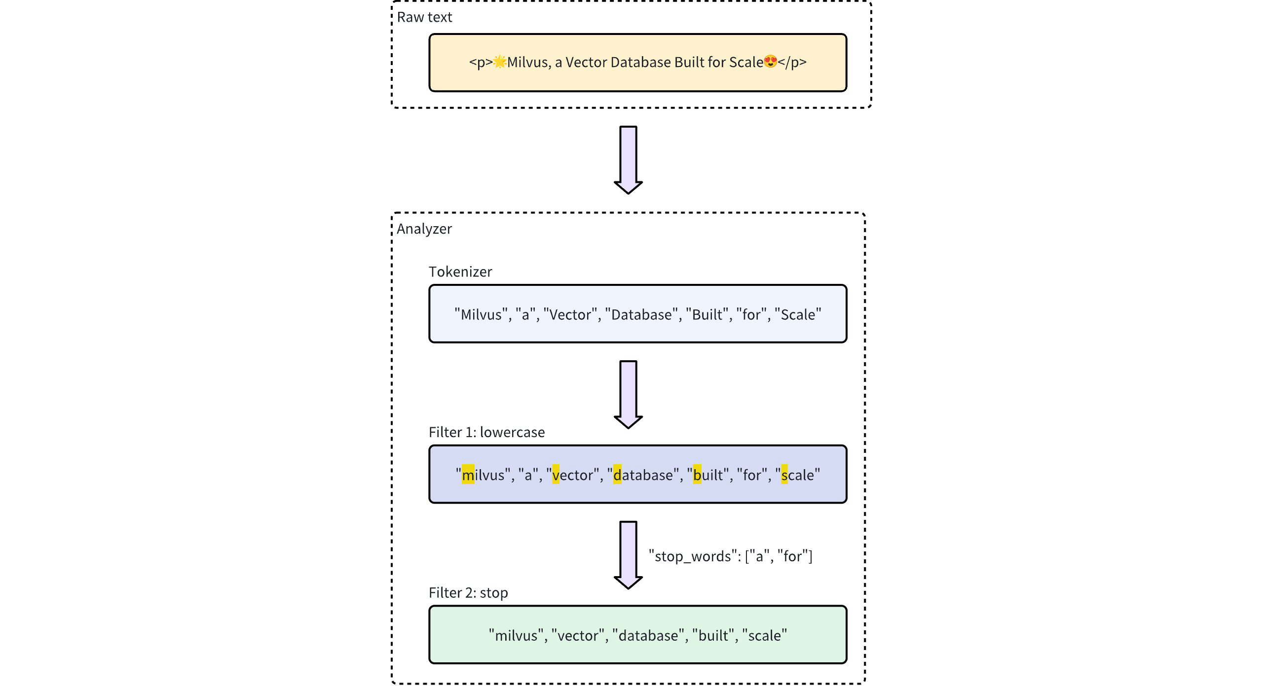
# Analyzer types
Milvus provides two types of analyzers to meet different text processing needs:
- Built-in analyzer: These are predefined configurations that cover common text processing tasks with minimal setup. Built-in analyzers are ideal for general-purpose searches, as they require no complex configuration.
- Custom analyzer: For more advanced requirements, custom analyzers allow you to define your own configuration by specifying both the tokenizer and zero or more filters. This level of customization is especially useful for specialized use cases where precise control over text processing is needed.
NOTE
- If you omit analyzer configurations during collection creation, Milvus uses the
standardanalyzer for all text processing by default. For details, refer to Standard Analyzer. - For optimal search and query performance, choose an analyzer that matches the language of your text data. For instance, while the
standardanalyzer is veratile, it may not be the best choice for languages with unique grammatical structures, such as Chinese, Japanese, or Korean. In such cases, using a language specific analyzer likechineseor custom analyzers with specialized tokenizers (such aslindera,icu) and filters is highly recommended to ensure accurate tokenization and better search results.
# Built-in analyzer
Built-in analyzers in Milvus are pre-configured with specific tokenizers and filters, allowing you to use them immediately without needing to define these components yourself. Each built-in analyzer serves as a template that includes a preset tokenizer and filters, with optional parameters for customization.
For example, to use the standard built-in analyzer, simply specify its name standard as the type and optionally include extra configurations specific to this analyzer type, such as stop_words:
analyzer_params = {
    "type": "standard" # Uses the standard built-in analyzer
    "stop_words": ["a", "an", "for"] # Defines a list of common words (stop words) to exclude from tokenization
}
2
3
4
To check the execution result of an analyzer, use the run_analyzer method:
# Sample text to analyze
text = "An efficient system relies on a robust analyzer to correctly process text for various applications."

# Run analyzer
result = client.run_analyzer(
    text,
    analyzer_params
)
2
3
4
5
6
7
8
The output will be:
['efficient', 'system', 'relies', 'on', 'robust', 'analyzer', 'to', 'correctly', 'process', 'text', 'various', 'applications']
This demonstrates that the analyzer properly tokenizes the input text by filtering out the stop words "a", "an", and "for", while returning the remaining meaningful tokens.
The configuration of the standard built-in analyzer above is equivalent to setting up a custom analyzer with the following parameters, where tokenizer and filter options are explicitly defined to achieve similar functionality:
analyzer_params = {
    "tokenizer": "standard",
    "filter": [
        "lowercase",
        {
            "type": "stop",
            "stop_words": ["a", "an", "for"]
        }
    ]
}
2
3
4
5
6
7
8
9
10
Milvus offers the following built-in analyzers, each designed for specific text processing needs:
standard: Suitable for general-purpose text processing, applying standard tokenization and lowercase filtering.english: Optimized for English-language text, with support for English stop words.chinese: Specialized for processing Chinese text, including tokenization adapted for Chinese language structures.
# Custom analyzer
For more advanced text processing, custom analyzers in Milvus allow you to build a tailored text-handling pipeline by specifying both a tokenizer and filters. This setup is ideal for specialized use cases where precise control is required.
Tokenizer:
The tokenizer is a mandatory component for a custom analyzer, which initiates the analyzer pipeline by breaking down input text into discrete units or tokens. Tokenization follows specific rules, such as splitting by whitespace or punctuation, depending on the tokenizer type. This process allows for more precise and independent handling of each word or phrase.
For example, a tokenizer would convert text "Vector Database Built for Scale" into separate tokens:
["Vector", "Database", "Built", "for", "Scale"]
Example of specifying a tokenizer:
analyzer_params = {
    "tokenizer": "whitespace"
}
2
3
filter:
Filters are optional components working on the tokens produced by the tokenizer, transforming or refining them as needed. For example, after applying a lowercase filter to the tokenized terms ["Vector", "Database", "Built", "for", "Scale"], the result might be:
["vector", "database", "built", "for", "scale"]
Filters in a custom analyzer can be either built-in or custom, depending on configuration needs.
- Built-in filters: Pre-configured by Milvus, requiring minimal setup. You can use these filters out-of-the-box by specifying their names. The filters below are built-in for direct use:
lowercase: Converts text to lowercase, ensuring case-insensitive matching. For details, refer to Lowercase.asciifolding: Converts non-ASCII characters to ASCII equivalents, simplifying multilingual text handling. For details, refer to ASCII folding.alphanumonly: Retains only alphanumeric characters by removing others. For details, refer to Alphanumonly.cnalphanumonly: Removes tokens that contain any characters other than Chinese characters, English letters, or digits. For details, refer to Cnalphanumonly.cncharonly: Removes tokens that contain any non-Chinese characters. For details, refer to Cncharonly.
Example of using a built-in filter:
analyzer_params = {
    "tokenizer": "standard", # Mandatory: Specifies tokenizer
    "filter": ["lowercase"], # Optional: Built-in filter that converts text to lowercase
}
2
3
4
- Custom filters: Custom filters allow for specialized configurations. You can define a custom filter by choosing a valid filter type (
filter.type) and adding specific settings for each filter type. Examples of filter types that support customization:stop: Removes specified common words by setting a list of stop words (e.g.,"stop_words": ["of", "to"]). For detail, refer to Stop.length: Excludes tokens based on length criteria, such as setting a maximum token length. For details, refer to Length.stemmer: Reduces words to their root forms for more flexible matching. For details, refer to Stemmer.
Example of configuring a custom filter:
analyzer_params = {
    "tokenizer": "standard", # Mandatory: Specifies tokenizer
    "filter": [
        {
            "type": "stop", # Specifies 'stop' as the filter type
            "stop_words": ["of", "to"], # Customizes stop words for this filter type
        }
    ]
}
2
3
4
5
6
7
8
9
# Example use
In this example, you will create a collection schema that includes:
- A vector field for embeddings.
- Two
VARCHARfields for text processing:- One field uses a built-in analyzer.
- The other uses a custom analyzer.
Before incorporating these configurations into your collection, you'll verify each analyzer using the run_analyzer method.
# Step 1: Initialize MilvusClient and create schema
Begin by setting up the Milvus client and creating a new schema.
from pymilvus import MilvusClient, DataType

# Set up a Milvus client
client = MilvusClient(uri="http://localhost:19530")

# Create a new schema
schema = client.create_schema(auto_id=True, enable_dynamic_field=False)
2
3
4
5
6
7
# Step 2: Define and verify analyzer configurations
- Configure and verify a built-in analyzer (
english):- Configuration: Define the analyzer parameters for the built-in English analyzer.
- Verification: Use
run_analyzerto check that the configuration produces the expected tokenization.
# Built-in analyzer configuration for English text processing
analyzer_params_built_in = {
    "type": "english"
}

# Verify built-in analyzer configuration
sample_text = "Milvus simplifies text analysis for search."
result = client.run_analyzer(sample_text, analyzer_params_built_in)
print("Built-in analyzer output:", result)

# Expected output:
# Built-in analyzer output: ['milvus', 'simplifi', 'text', 'analysi', 'search']
2
3
4
5
6
7
8
9
10
11
12
- Configure and verify a custom analyzer:
- Configuration: Define a custom analyzer that uses a standard tokenizer along with a built-in lowercase filter and custom filters for token length and stop words.
- Verification: Use
run_analyzerto ensure the custom configuration processes text as intended.
# Custom analyzer configuration with a standard tokenizer and custom filters
analyzer_params_custom = {
    "tokenizer": "standard",
    "filter": [
        "lowercase", # Built-in filter: Convert tokens to lowercase
        {
            "type": "length", # Custom filter: restrict token length
            "max": 40
        },
        {
            "type": "stop", # Custom filter: remove specified stop words
            "stop_words": ["of", "for"]
        }
    ]
}

# Verify custom analyzer configuration
sample_text = "Milvus provides flexible, customizable analyzers for robust text processing."
result = client.run_analyzer(sample_text, analyzer_params_custom)
print("Custom analyzer output:", result)

# Expected output:
# Custom analyzer output: ['milvus', 'provides', 'flexible', 'customizable', 'analyzers', 'robust', 'text', 'processing']
2
3
4
5
6
7
8
9
10
11
12
13
14
15
16
17
18
19
20
21
22
23
# Step 3: Add fields to the schema
Now that you have verified your analyzer configurations, add them to your schema fields:
# Add VARCHAR field 'title_en' using the built-in analyzer configuration
schema.add_field(
    field_name='title_en',
    datatype=DataType.VARCHAR,
    max_length=1000,
    enable_analyzer=True,
    analyzer_params=analyzer_params_built_in,
    enable_match=True,
)

# Add VARCHAR field 'title' using the custom analyzer configuration
schema.add_field(
    field_name='title',
    datatype=DataType.VARCHAR,
    max_length=1000,
    enable_analyzer=True,
    analyzer_params=analyzer_params_custom,
    enable_match=True,
)

# Add a vector field for embeddings
schema.add_field(field_name="embedding", datatype=DataType.FLOAT_VECTOR, dim=3)

# Add a primary key field
schema.add_field(field_name="id", datatype=DataType.INT64, is_primary=True)
2
3
4
5
6
7
8
9
10
11
12
13
14
15
16
17
18
19
20
21
22
23
24
25
# Step 4: Prepare index parameters and create the collection
# Set up index parameters for the vector field
index_params = client.prepare_index_params()
index_params.add_index(field_name="embedding", metric_type="COSINE", index_type="AUTOINDEX")

# Create the collection with the defined schema and index parameters
client.create_collection(
    collection_name="my_collection",
    schema=schema,
    index_params=index_params
)
2
3
4
5
6
7
8
9
10
# Built-in Analyzers
# Standard
The standard analyzer is the default analyzer in Milvus, which is automatically applied to text fields if no analyzer is specifid. It uses grammar-based tokenization, making it effective for most languages.
NOTE
The standard analyzer is suitable for languages that rely on separators (such as spaces, punctuation) for word boundaries. However, languages like Chinese, Japanese, and Korean require dictionary-based tokenizations. In such cases, using a Language-specific analyzer like chinese or custom analyzers with specialized tokenizers (such as lindera, icu) and filters is highly recommended to ensure accurate tokenization and better search results.
# Definition
The standard analyzer consists of:
- Tokenizer: Uses the
standardtokenizer to split text into discrete word units based on grammar rules. For more information, refer to Standard Tokenizer. - Filter: Uses the
lowercasefilter to convert all tokens to lowercase, enabling case-insensitive searches. For more information, refer to Lowercase.
The functionality of the standard analyzer is equivalent to the following custom analyzer configuration:
analyzer_params = {
    "tokenizer": "standard",
    "filter": ["lowercase"]
}
2
3
4
# Configuration
To apply the standard analyzer to a field, simply set type to standard in analyzer_params, and include optional parameters as needed.
analyzer_params = {
    "type": "standard", # Specifies the standard analyzer type
}
2
3
The standard analyzer accepts the following optional parameters:
| Parameter | Description |
|---|---|
stop_words | An array containing a list of stop words, which will be removed from tokenization. Defaults to _english_, a built-in set of common English stop words. |
Example configuration of custom stop words:
analyzer_params = {
    "type": "standard", # Specifies the standard analyzer type
    "stop_words": ["of"] # Optional: List of words to exclude from tokenization
}
2
3
4
After defining analyzer_params, you can apply them to a VARCHAR field when defining a collection schema. This allows Milvus to process the text in that field using the specified analyzer for efficient tokenization and filtering. For more information, refer to Example use.
# Examples
Before applying the analyzer configuration to your collection schema, verify its behavior using the run_analyzer method.
- Analyzer configuration:
analyzer_params = {
    "type": "standard", # Standard analyzer configuration
    "stop_words": ["for"] # Optional: Custom stop words parameter
}
2
3
4
- Verification using run_analyzer:
from pymilvus import (
    MilvusClient,
)

client = MilvusClient(
    uri="http://localhost:19530",
    token="root:Milvus"
)

# Sample text to analyze
sample_text = "The Milvus vector database is built for scale!"

# Run the standard analyzer with the defined configuration
result = client.run_analyzer(sample_text, analyzer_params)
print("Standard analyzer output:", result)
2
3
4
5
6
7
8
9
10
11
12
13
14
15
- Expected output:
Standard analyzer output: ['the', 'milvus', 'vector', 'database', 'is', 'built', 'scale']
# English
The english analyzer in Milvus is designed to process English text, applying language-specific rules for tokenization and filtering.
# Definition
The english analyzer uses the following components:
- Tokenizer: Uses the
standardtokenizer to split text into discrete word units. - Filters: Includes multiple filters for comprehensive text processing:
lowercase: Converts all tokens to lowercase, enabling case-insensitive searches.stemmer: Reduces words to their root form to support broader matching (e.g., "running" becomes "run").stop_words: Removes common English stop words to focus on key terms in text.
The functionality of the english analyzer is equivalent to the following custom analyzer configuration:
analyzer_params = {
    "tokenizer": "standard",
    "filter": [
        "lowercase",
        {
            "type": "stemmer",
            "language": "english"
        },
        {
            "type": "stop",
            "stop_words": "_english_"
        }
    ]
}
2
3
4
5
6
7
8
9
10
11
12
13
14
# Configuration
To apply the english analyzer to a field, simply set type to english in analyzer_params, and include optional parameters as needed.
analyzer_params = {
    "type": "english"
}
2
3
The english analyzer accepts the following optional parameters:
| Parameter | Description |
|---|---|
stop_words | An array containing a list of stop words, which will be removed from tokenization. Defaults to _english_, a built-in set of common English stop words. |
Example configuration with custom stop words:
analyzer_params = {
    "type": "english",
    "stop_words": ["a", "an", "the"]
}
2
3
4
After defining analyzer_params, you can apply them to a VARCHAR field when defining a collection schema. This allows Milvus to process the text in that field using the specified analyzer for efficient tokenization and filtering. For details, refer to Example use.
# Examples
Before applying the analyzer configuration to your collection schema, verify its behavior using the run_analyzer method.
- Analyzer configuration
analyzer_params = {
    "type": "english",
    "stop_words": ["a", "an", "the"]
}
2
3
4
- Verification using run_analyzer
from pymilvus import (
    MilvusClient,
)

client = MilvusClient(uri="http://localhost:19530")

# Sample text to analyze
sample_text = "Milvus is a vector database built for scale!"

# Run the standard analyzer with the defined configuration
result = client.run_analyzer(sample_text, analyzer_params)
print("English analyzer output:", result)
2
3
4
5
6
7
8
9
10
11
12
- Expected output
English analyzer output: ['milvus', 'vector', 'databas', 'built', 'scale']
# Chinese
The chinses analyzer is designed specifically to handle Chinese text, providing effective segmentation and tokenization.
# Definition
The chinese analyzer consists of:
- Tokenizer: Uses the
jiebatokenizer to segment Chinese text into tokens based on vocabulary and context. For more information, refer to Jieba. - Filter: Uses the
cnalphanumonlyfilter to remove tokens that contain any non-Chinese characters. For more information, refer to Cnalphanumonly.
The functionality of the chinese analyzer is equivalent to the following custom analyzer configuration:
analyzer_params = {
    "tokenizer": "jieba",
    "filter": ["cnalphanumonly"]
}
2
3
4
# Configuration
To apply the chinese analyzer to a field, simply set type to chinese in analyzer_params.
analyzer_params = {
    "type": "chinese",
}
2
3
NOTE
The chinese analyzer does not accept any optional parameters.
# Examples
Before applying the analyzer configuration to your collection schema, verify its behavior using the run_analyzer method.
- Analyzer configuration
analyzer_params = {
    "type": "chinese",
}
2
3
- Verification using run_analyzer
from pymilvus import (
    MilvusClient,
)

client = MilvusClient(uri="http://localhost:19530")

# Sample text to analyze
sample_text = "Milvus 是一个高性能, 可扩展的向量数据库!"

# Run the standard analyzer with the defined configuration
result = client.run_analyzer(sample_text, analyzer_params)
print("English analyzer output:", result)
2
3
4
5
6
7
8
9
10
11
12
- Expected output
Chinese analyzer output: ['Milvus', '是', '一个', '高性', '性能', '高性能', '可', '扩展', '的', '向量', '数据', '据库', '数据库']
# Tokenizers
# Standard
The standard tokenizer in Milvus splits text based on spaces and punctuation marks, making it suitable for most languages.
# Configuration
To configure an analyzer using the standard tokenizer, set tokenizer to standard in analyzer_params.
analyzer_params = {
    "tokenizer": "standard"
}
2
3
The standard tokenizer can work in conjunction with one or more filters. For example, the following code defines an analyzer that uses the standard tokenizer and lowercase filter:
analyzer_params = {
    "tokenizer": "standard",
    "filter": ["lowercase"]
}
2
3
4
NOTE
For simpler setup, you may choose to use the standard analyzer, which combines the standard tokenizer with the lowercase filter.
After defining analyzer_params, you can apply them to a VARCHAR field when defining a collection schema. This allows Milvus to process the text in that field using the specified analyzer for efficient tokenization and filtering. For details, refer to Example use.
# Examples
Before applying the analyzer configuration to your collection schema, verify its behavior using the run_analyzer method.
- Analyzer configuration
analyzer_params = {
    "tokenizer": "standard",
    "filter": ["lowercase"]
}
2
3
4
- Verification using run_analyzer
from pymilvus import (
    MilvusClient,
)

client = MilvusClient(
    uri="http://localhost:19530",
    token="root:Milvus"
)

# Sample text to analyze
sample_text = "The Milvus vector database is built for scale!"

# Run the standard analyzer with the defined configuration
result = client.run_analyzer(sample_text, analyzer_params)
print("English analyzer output:", result)
2
3
4
5
6
7
8
9
10
11
12
13
14
15
- Expected output
['the', 'milvus', 'vector', 'database', 'is', 'built', 'for', 'scale']
# Whitespace
The whitespace tokenizer divides text into terms whenever there is a space between words.
# Configuration
To configure an analyzer using the whitespace tokenizer, set tokenizer to whitespace in analyzer_params.
analyzer_params = {
    "tokenizer": "whitespace",
}
2
3
The whitespace tokenizer can work in conjunction with one or more filters. For example, the following code defines an analyzer that uses the whitespace tokenizer and lowercase filter:
analyzer_params = {
    "tokenizer": "whitespace",
    "filter": ["lowercase"]
}
2
3
4
After defining analyzer_params, you can apply them to a VARCHAR field when defining a collection schema. This allows Milvus to process the text in the field using the specified analyzer for efficient tokenization and filtering. For details, refer to Example use.
# Examples
Before applying the analyzer configuration to your collection schema, verify its behavior using the run_analyzer method.
- Analyzer configuration
analyzer_params = {
    "tokenizer": "whitespace",
    "filter": ["lowercase"]
}
2
3
4
- Verification using run_analyzer
from pymilvus import (
    MilvusClient,
)

client = MilvusClient(uri="http://localhost:19530")

# Sample text to analyze
sample_text = "The Milvus vector database is built for scale!"

# Run the standard analyzer with the defined configuration
result = client.run_analyzer(sample_text, analyzer_params)
print("Standard analyzer output:", result)
2
3
4
5
6
7
8
9
10
11
12
- Expected output
['the', 'milvus', 'vector', 'database', 'is', 'built', 'for', 'scale!']
# Jieba
The jieba tokenizer processes Chinese text by breaking it down into its component words.
NOTE
The jieba tokenizer preserves punctuation marks as separate tokens in the output. For example, "你好!世界。" becomes ["你好", "!", "世界", "。"]. To remove these standalone punctuation tokens, use the removepunct filter.
# Configuration
Milvus supports two configuration approaches for the jieba tokenizer: a simple configuration and a custom configuration.
- Simple configuration
With the simple configuration, you only need to set the tokenizer to "jieba". For example:
# Simple configuration: only specifying the tokenizer name
analyzer_params = {
    "tokenizer": "jieba", # Use the default settings: dict=["_default_"], mode="search", hmm=True
}
2
3
4
This simple configuration is equivalent to the following custom configuration:
# Custom configuration equivalent to the simple configuration above
analyzer_params = {
    "type": "jieba", # Tokenizer type, fixed as "jieba"
    "dict": ["_default_"], # Use the default dictionary
    "mode": "search", # Use search mode for improved recall (see mode details)
    "hmm": True # Enable HMM for probabilistic segmentation
}
2
3
4
5
6
7
For details on parameters, refer to Custom configuration.
- Custom configuration
For more control, you can provide a custom configuration that allows you to specify a custom dictionary, select the segmentation mode, and enable or disable the Hidden Markov Model (HMM). For example:
# Custom configuration with user-defined settings
analyzer_params = {
    "tokenizer": {
        "type": "jieba", # Fixed tokenizer type
        "dict": ["customDictionary"], # Custom dictionary list; replace with your own terms
        "mode": "exact", # Use exact mode (non-overlapping tokens)
        "hmm": False # Disable HMM; unmatched text will be split into individual characters
    }
}
2
3
4
5
6
7
8
9
| Parameter | Description | Default Value |
|---|---|---|
type | The type of tokenizer. This is fixed to "jieba" | "jieba" |
dict | A list of dictionaries that the analyzer will load as its vocabulary source. Built-in options: 1. "_default_": Loads the engine's built-in Simplified-Chinese dictionary. For details, refer to dict.txt 2. "_extend_default_": Loads everything in "_default_" plus an additional Traditional-Chinese supplement. For details, refer to dict.txt.big. You can also mix the built-in dictionary with any number of custom dictionaries. Example: ["_default_", "结巴分词器"] | ["_default_"] |
mode | The segmentation mode. Possible values: 1. "exact": Tries to segment the sentence in the most precise manner, making it ideal for text analysis. 2. "search": Builds on exact mode by further breaking down long words to improve recall, making it suitable for search engine tokenization. For more information, refer to Jieba GitHub Project. | "search" |
hmm | A boolean flag indicating whether to enable the Hidden Markov Model (HMM) for probabilistic segmentation of words not found in the dictionary. | True |
After defining analyzer_params, you can apply them to a VARCHAR field when defining a collection schema. This allows Milvus to process the text in that field using the specified analyzer for efficient tokenization and filtering. For details, refer to Example use.
# Examples
Before applying the analyzer configuration to your collection schema, verify its behavior using the run_analyzer method.
- Analyzer configuration
analyzer_params = {
    "tokenizer": {
        "type": "jieba",
        "dict": ["结巴分词器"],
        "mode": "exact",
        "hmm": False
    }
}
2
3
4
5
6
7
8
- Verification using run_analyzer
from pymilvus import (
    MilvusClient,
)

client = MilvusClient(uri="http://localhost:19530")

sample_text = "milvus结巴分词器中文测试"

result = client.run_analyzer(sample_text, analyzer_params)
print("Standard analyzer output:", result)
2
3
4
5
6
7
8
9
10
- Expected output
['milvus', '结巴分词器', '中', '文', '测', '试']
# Lindera
The lindera tokenizer performs dictionary-based morphological analysis. It is a good choice for languages-such as Japanese, Korean, and Chinese -- Whose words are not separated by spaces.
NOTE
The lindera tokenizer preserves punctuation marks as separate tokens in the output. For example, "こんにちは!" becomres ["こんにちは", "!"]. To remove these standalone punctuation tokens, use the removepunct filter.
# Prerequisites
To use the lindera tokenizer, you need to use a specially compiled Milvus version. All dictionaries must be explicitly enabled during compilation to be used.
To enable specific dictionaries, include them in the compilation command:
make milvus TANTIVY_FEATURES=lindera-ipadic,lindera-ko-dic
The complete list of available dictionaries is: lindera-ipadic, lindera-ipadic-neologd, lindera-unidic, lindera-ko-dic, lindera-cc-cedict.
For example, to enable all dictionaries:
make milvus TANTIVY_FEATURES=lindera-ipadic,lindera-ipadic-neologd,lindera-unidic,lindera-ko-dic,lindera-cc-cedict
# Configuration
To configure an analyzer using the lindera tokenizer, set tokenizer.type to lindera and choose a dictionary with dict_kind.
analyzer_params = {
    "tokenizer": {
        "type": "lindera",
        "dict_kind": "ipadic"
    }
}
2
3
4
5
6
| Parameter | Description |
|---|---|
type | The type of tokenizer. This is fixed to "lindera". |
dict_kind | A dictionary used to define vocabulary. Possible values: 1. ko_dic: Korean - Korean morphological dictionary (MeCab Ko-dic) 2. ipadic: Japanese - Standard morphological dictionary (MeCab IPADIC) 3. ipadic-neologd: Janpanese with neologism dictionary (extended) - Includes new words and proper nouns (IPADIC NEologd) 4. unidic: Japanese UniDic (extended) - Academic standard dictionary with detailed linguistic information (UniDic) 5. cc-cedict: Mandarin Chinese (traditional/simplified) - Community-maintained Chinese-English dictionary (CC-CEDICT) Note: All dictionaries must be enabled during Milvus compilation to be available for use. |
After defining analyzer_params, you can apply them to a VARCHAR field when defining a collection schema. This allows Milvus to process the text in that field using the specified analyzer for efficient tokenization and filtering. For details, refer to Example use.
# Examples
Before applying the analyzer configuration to your collection schema, verify its behavior using the run_analyzer method.
- Analyzer configuration
analyzer_params = {
    "tokenizer": {
        "type": "linera",
        "dict_kind": "ipadic"
    }
}
2
3
4
5
6
- Verification using run_analyzer
from pymilvus import (
    MilvusClient,
)

client = MilvusClient(uri="http://localhost:19530")

# Sample text to analyze
sample_text = "東京スカイツリーの最寄り駅はとうきょうスカイツリー駅で"

# Run the standard analyzer with the defined configuration
result = client.run_analyzer(sample_text, analyzer_params)
print("Standard analyzer output:", result)
2
3
4
5
6
7
8
9
10
11
12
- Expected output
{tokens: ['東京', 'スカイ', 'ツリー', 'の', '最寄り駅', 'は', 'とう', 'きょう', 'スカイ', 'ツリー', '駅', 'で']}
# ICU
The icu tokenizer is built on the Internationalization Components of Unicode(ICU) open-source project, which provides key tools for software internationalization. By using ICU's word-break algorithm, the tokenizer can accurately split text into words across the majority of the world's languages.
NOTE
The icu tokenizer preserves punctuation marks and spaces as separate tokens in the output. For example, "Привет! Как дела?" becomes ["Привет", "!", " ", "Как", " ", "дела", "?"]. To remove these standalone punctuation tokens, use the removepunct filter.
# Configuration
To configure an analyzer using the icu tokenizer, set tokenizer to icu in analyzer_params.
analyzer_params = {
    "tokenizer": "icu",
}
2
3
The icu tokenizer can work in conjunction with one or more filters. For example, the following code defines an analyzer that uses the icu tokenizer and remove punct filter:
analyzer_params = {
    "tokenizer": "icu",
    "filter": ["removepunct"]
}
2
3
4
After defining analyzer_params, you can apply them to a VARCHAR field when defining a collection schema. This allows Milvus to process the text in that field using the specified analyzer for efficient tokenization and filtering. For details, refer to Example use.
# Examples
Before applying the analyzer configuration to your collection schema, verify its behavior using the run_analyzer method.
- Analyzer configuration
analyzer_params = {
    "tokenizer": "icu",
}
2
3
- Verification using run_analyzer
from pymilvus import (
    MilvusClient,
)

client = MilvusClient(uri="http://localhost:19530")

# Sample text to analyze
sample_text = "Привет! Как дела?"

# Run the standard analyzer with the defined configuration
result = client.run_analyzer(sample_text, analyzer_params)
print("Standard analyzer output:", result)
2
3
4
5
6
7
8
9
10
11
12
- Expected output
['Привет', '!', ' ', 'Как', ' ', 'дела', '?']
# Language Identifier
The language_identifier is a specialized tokenizer designed to enhance the text search capabilities of Milvus by automating the language analysis process. Its primary function is to detect the language of a text field and then dynamically apply a pre-configured analyzer that is most suitable for that language. This is particularly valuable for applications that handle a variety of languages, as it eliminates the need for manual language assignment on a per-input basis.
By intelligently routing text data to the appropriate processing pipeline, the language_identifier streamlines multilingual data ingestion and ensures accurate tokenization for subsequent search and retrieval operations.
# Language detection workflow
The language_identifier performs a series of steps to process a text string, a workflow that is critical for users to understand how to configure it correctly.

- Input: The workflow begins with a text string as input.
- Language detection: This string is first passed to a language detection engine, which attempts to identify the language. Milvus supports two engines: whatlang and lingua.
- Analyzer selection:
- Success: If the language is successfully detected, the system checks if the detected language name has a corresponding analyzer configured in your
analyzersdictionary. If a match is found, the system applies the specified analyzer to the input text. For example, a detected "Mandarin" text would be routed to ajiebatokenizer. - Fallback: If detection fails, or if a language is successfully detected but you have not provided a specific analyzer for it, the system defaults to a pre-configured default analyzer. This is a crucial point of clarification; the
defaultanalyzer is a fallback for both detection failure and an absence of a matching analyzer.
- Success: If the language is successfully detected, the system checks if the detected language name has a corresponding analyzer configured in your
After the appropriate analyzer is chosen, the text is tokenized and processed, completing the workflow.
# Available language detection engines
Milvus offers a choice between two language detection engines:
The selection depends on the specific performance and accuracy requirements of your application.
| Engine | Speed | Accuracy | Output Format | Best For |
|---|---|---|---|---|
whatlang | Fast | Good for most languages | Language names (e.g., English, Mandarin, Japanese) Reference: Language column in supported languages table | Real-time applications where speed is critical |
lingua | Slower | Higher precision, especially for short texts | English language names (e.g., English, Chinese, Japanese) Reference: Supported languages list | Applications where accuracy is more important than speed |
A critical consideration is the engine's naming convention. While both engines return language names in English, they use different terms for some languages (e.g., whatlang returns Mandarin, while lingua returns Chinese). The analyzer's key mus be an exact match to the name returned by the chosen detection engine.
# Configuration
To correctly use the language_identifier tokenizer, the following steps must be taken to define and apply its configuration.
- Step 1: Choose your languages and analyzers
The core of setting up the language_identifier is tailoring your analyzers to the specific languages you plan to support. The system works by matching the detected language with the correct analyzer, so this step is crucial for accurate text processing.
Below is a recommended mapping of languages to suitable Milvus analyzers. This table serves as a bridge between the output of the language detection engine and the best tool for the job.
| Language (Detector Output) | Recommended Analyzer | Description |
|---|---|---|
English | type: english | Standard English tokenizatio with stemming and stop-word fitering. |
Mandarin(Via whatlang) or Chinese(via lingua) | tokenizer: jieba | Chinese word segmentation for non-space-delimited text. |
Japanese | tokenizer: icu | A robust tokenizer for complex scripts, including Japanese. |
French | type: standard, filter: ["lowercase", "asciifolding"] | A custom configuration that handles French accents and characters. |
NOTE
- Matching is Key: The name of your analyzer must exactly match the language output of the detection engine. For instance, if you're using
whatlang, the key for Chinese text must beMandarin. - Best practices: The table above provides recommended configurations for a few common languages, but it is not an exhaustive list. For a more comprehensive guide on choosing analyzers, refer to Choose the Right Analyzer for Your Use Case.
- Detector output: For a complete list of language names returned by the detection engines, refer to Whatlang supported languages table and the Lingua supported languages list.
- Step 2: Define analyzer_params
To use the language_identifier tokenizer in Milvus, create a dictionary containing these key components:
Required components:
analyzersconfig set -- A dictionary containing all analyzer configurations, which must include:default-- The fallback analyzer used when language detection fails or no matching analyzer is found- Language-specific analyzers -- Each defined as
<analyzer_name>: <analyzer_config>, where:analyzer_namematches your chosen detection engine's output (e.g.,"English","Japanese")analyzer_configfollows standard analyzer parameter format (see Analyzer Overview)
Optional components:
identifier-- Specifies which language detection engine to use (whatlangorlingua). Defaults towhatlangif not specifiedmapping-- Creates custom aliases for your analyzers, allowing you to use descriptive names instead of the detection engine's exact output format.
The tokenizer works by first detecting the language of input text, then selecting the appropriate analyzer from your configuration. If detection fails or no matching analyzer exists, it automatically falls back to your default analyzer.
Recommended: Direct name matching:
Your analyzer names should exactly match the output of your chosen language detection engine. This approach is simpler and avoids potential confusion.
For both whatlang and lingua, use the language names as shown in their respective documentation:
- whatlang supported languages (use the "Language" column)
- lingua supported languages
analyzer_params = {
    "tokenizer": {
        "type": "language_identifier", # Must be `language_identifier`
        "identifier": "whatlang", # or `lingua`
        "analyzers": { # A set of analyzer configs
            "default": {
                "tokenizer": "standard" # fallback if language detection fails
            },
            "English": { # Analyzer name that matches whatlang output
                "type": "english"
            },
            "Mandarin": { # Analyzer name that matches whatlang output
                "tokenizer": "jieba"
            }
        }
    }
}
2
3
4
5
6
7
8
9
10
11
12
13
14
15
16
17
Alternative approach: Custom names with mapping:
If you prefer to use custom analyzer names or need to maintain compatibility with existing configurations, you can use the mapping parameter. This creates aliases for your analyzers -- both the original detection engine names and your custom names will work.
analyzer_params = {
    "tokenizer": {
        "type": "language_identifier",
        "identifier": "lingua",
        "analyzers": {
            "default": {
                "tokenizer": "standard"
            },
            "english_analyzer": { # Custom analyzer name
                "type": "english"
            },
            "chinese_analyzer": { # Custom analyzer name
                "tokenizer"; "jieba"
            }
        },
        "mapping": {
            "English": "english_analyzer", # Maps detection output to custom name
            "Chinese": "chinese_analyzer"
        }
    }
}
2
3
4
5
6
7
8
9
10
11
12
13
14
15
16
17
18
19
20
21
After defining analyzer_params, you can apply them to a VARCHAR field when defining a collection schema. This allows Milvus to process the text in that field using the specified analyzer for efficient tokenization and filtering. For details, refer to Example use.
# Examples
Here are some ready-to-use configurations for common scenarios. Each example includes both the configuration and verification code so you can test the setup immediately.
- English and Chinese detection
from pymilvus import MilvusClient

# Configuration
analyzer_params = {
    "tokenizer": {
        "type": "language_identifier",
        "identifier": "whatlang",
        "analyzers": {
            "default": {"tokenizer": "standard"},
            "English": {"type": "english"},
            "Mandarin": {"tokenizer": "jieba"}
        }
    }
}

# Test the configuration
client = MilvusClient(
    uri="http://localhost:19530",
    token="root:Milvus"
)

# English text
result_en = client.run_analyzer("The Milvus vector database is built for scale!", analyzer_params)
print("English": result_en)
# Output
# English: ['The', 'Milvus', 'vector', 'database', 'is', 'built', 'for', 'scale']

# Chinese text
result_cn = client.run_analyzer("Milvus向量数据库专为大规模应用而设计", analyzer_params)
print("Chinese:", result_cn)
# Output
# Chinese: ['Milvus', '向量', '数据', '据库', '数据库', '专', '为', '大规', '规模', '大规模', '应用', '而', '设计']
2
3
4
5
6
7
8
9
10
11
12
13
14
15
16
17
18
19
20
21
22
23
24
25
26
27
28
29
30
31
32
- European languages with accent normalization
# Configuration for French, German, Spanish, etc.
analyzer_params = {
    "tokenizer": {
        "type": "language_identifier",
        "identifier": "lingua",
        "analyzers": {
            "default": {"tokenizer": "standard"},
            "English": {"type": "english"},
            "French": {
                "tokenizer": "standard",
                "filter": ["lowercase", "asciifolding"]
            }
        }
    }
}

# Test with accented text
result_fr = client.run_analyzer("Café français très délicieux", analyzer_params)
print("French:", result_fr)
# Output:
# French: ['cafe', 'francais', 'tres', 'delicieux']
2
3
4
5
6
7
8
9
10
11
12
13
14
15
16
17
18
19
20
21
# Usage notes
- Single-language per field: It operates on a field as a single, homogenous unit of text. It is designed to handle different languages across different data records, such as one record containing an English sentence and the next containing a French sentence.
- No mixed-language strings: It is not designed to handle a single string that contains text from multiple languages. For example, a single
VARCHARfield containing both an English sentence and a quoted Japanese phrase will be processed as a single language. - Dominant language processing: In mixed-language scenarios, the detection engine will likely identify the dominant language, and the corresponding analyzer will be applied to the entire text. This will result in poor or no tokenization for the embedded foreign text.
# Filters
# Lowercase
The lowercase filter converts terms generated by a tokenizer to lowercase, making searches case-insensitive. For example, it can convert ["High", "Performance", "Vector", "Database"] to ["high", "performance", "vector", "database"].
# Configuration
The lowercase filter is built into Milvus. To use it, simply specify its name in the filter section within analyzer_params.
analyzer_params = {
    "tokenizer": "standard",
    "filter": ["lowercase"],
}
2
3
4
The lowercase filter operates on the terms generated by the tokenizer, so it must be used in combination with a tokenizer.
After defining analyzer_params, you can apply them to a VARCHAR field when defining a collection schema. This allows Milvus to process the next in that field using the specified analyzer for efficient tokenization and filtering. For details, refer to Example use.
# Examples
Before applying the analyzer configuration to your collection schema, verify its behavior using the run_analyzer method.
- Analyzer configuration
analyzer_params = {
    "tokenizer": "standard",
    "filter": ["lowercase"],
}
2
3
4
- Verification using run_analyzer
from pymilvus import (
    MilvusClient,
)

client = MilvusClient(uri="http://localhost:19530")

# Sample text to analyze
sample_text = "The Lowercase Filter Ensures Uniformity In Text Processing."

# Run the standard analyzer with the defined configuration
result = client.run_analyzer(sample_text, analyzer_params)
print("Standard analyzer output:", result)
2
3
4
5
6
7
8
9
10
11
12
- Expected output
['the', 'lowercase', 'filter', 'ensures', 'uniformity', 'in', 'text', 'processing']
# ASCII Folding
The asciifolding filter converters outside the Basic Latin Unicode block(the first 127 ASCII character) into their ASCII equivalents. For instance, it transforms characters like í to i, making text processing simpler and more consistent, especially for multilingual content.
# Configuration
The asciifolding filter is built into Milvus. To use it, simply specify its name in the filter section within analyzer_params.
analyzer_params = {
    "tokenizer": "standard",
    "filter": ["asciifolding"],
}
2
3
4
The asciifolding filter operates on the terms generated by the tokenizer, so it must be used in combination with a tokenizer. For a list of tokenizers available in Milvus, refer to Standard Tokenizer and its sibling pages.
After defining analyzer_params, you can apply them to a VARCHAR field when defining a collection schema. This allows Milvus to process the text in that field using the specified analyzer for efficient tokenization and filtering. For details, refer to Example use.
# Examples
Before applying the analyzer configuration to your collection schema, verify its behavior using the run_analyzer method.
- Analyzer configuration
analyzer_params = {
    "tokenizer": "standard",
    "filter": ["asciifolding"],
}
2
3
4
- Verification using run_analyzer
from pymilvus import (
    MilvusClient,
)

client = MilvusClient(uri="http://localhost:19530")

# Sample text to analyze
sample_text = "Café Möller serves crème brûlée and piñatas."

# Run the standard analyzer with the defined configuration
result = client.run_analyzer(sample_text, analyzer_params)
print("Standard analyzer output:", result)
2
3
4
5
6
7
8
9
10
11
12
- Expected output
['Cafe', 'Moller', 'serves', 'creme', 'brulee', 'and', 'pinatas']
# Alphanumonly
The alphanumonly filter removes tokens that contain non-ASCII characters, keeping only alphanumeric terms. This filter is useful for processing text where only basic letters and numbers are relevant, excluding any special characters or symbols.
# Configuration
The alphanumonly filter is built into Milvus. To use it, simply specify its name in the filter section within analyzer_params.
analyzer_params = {
    "tokenizer": "standard",
    "filter": ["alphanumonly"],
}
2
3
4
The alphanumonly filter operates on the terms generated by the tokenizer, so it must be used in combination with a tokenizer. For a list of tokenizers available in Milvus, refer to Standard Tokenizer and its sibling pages.
After defining analyzer_params, you can apply them to a VARCHAR field when defining a collection schema. This allows Milvus to process the text in that field using the specified analyzer for efficient tokenization and filtering. For details, refer to Example use.
# Examples
Before applying the analyzer configuration to your collection schema, verify its behavior using the run_analyzer method.
- Analyzer configuration
analyzer_params = {
    "tokenizer": "standard",
    "filter": ["alphanumonly"],
}
2
3
4
- Verification using run_analyzer
from pymilvus import (
    MilvusClient,
)

client = MilvusClient(uri="http://localhost:19530")

# Sample text to analyzer
sample_text = "Milvus 2.0 @ Scale! #AI #Vector_Databasé"

# Run the standard analyzer with the defined configuration
result = client.run_analyzer(sample_text, analyzer_params)
print("Standard analyzer output:", result)
2
3
4
5
6
7
8
9
10
11
12
- Expected output
['Milvus', '2', '0', 'Scale', 'AI', 'Vector']
# Cnalphanumonly
The cnalphanumonly filter removes tokens that contain any characters other than Chinese characters, English letters, or digits.
# Configuration
The cnalphanumonly filter is built into Milvus. To use it, simply specify its name in the filter section within analyzer_params.
analyzer_params = {
    "tokenizer": "jieba",
    "filter": ["cnalphanumonly"],
}
2
3
4
The cnalphanumonly filter operates on the terms generated by the tokenizer, so it must be used in combination with a tokenizer. For a list of tokenizers available in Milvus, refer to Jieba and its sibling pages.
After defining analyzer_params, you can apply them to a VARCHAR field when defining a collection schema. This allows Milvus to process the text in that field using the specified analyzer for efficient tokenization and filtering. For details, refer to Example use.
# Examples
Before applying the analyzer configuration to your collection schema, verify its behavior using the run_analyzer method.
- Analyzer configuration
analyzer_params = {
    "tokenizer": "jieba",
    "filter": ["cnalphanumonly"]
}
2
3
4
- Verification using run_analyzer
from pymilvus import (
    MilvusClient,
)

client = MilvusClient(uri="http://localhost:19530")

# Sample text to analyze
sample_text = "Milvus 是 LF AI & Data Foundation 下的一个开源项目, 以 Apache 2.0 许可发布。"

# Run the jieba tokenizer with the defined configuration
result = client.run_analyzer(sample_text, analyzer_params)
print("Analyzer output:", result)
2
3
4
5
6
7
8
9
10
11
12
- Expected output
['Milvus', '是', 'LF', 'AI', 'Data', 'Foundation', '下的一个开源项目', '以', 'Apache', '2', '0', '许可发布']
# Cncharonly
The cncharonly filter removes tokens that contain any non-Chinese characters. This filter is useful when you want to focus solely on Chinese text, filtering out any tokens that contain other scripts, numbers, or symbols.
# Configuration
The cncharonly filter is built into Milvus. To use it, simply specify its name in the filter section within analyzer_params.
analyzer_params = {
    "tokenizer": "jieba",
    "filter": ["cncharonly"],
}
2
3
4
The cncharonly filter operates on the terms generated by the tokenizer, so it must be used in combination with a tokenizer. For a list of tokenizers available in Milvus, refer to Jieba and its sibling pages.
After defining analyzer_params, you can apply them to a VARCHAR field when defining a collection schema. This allows Milvus to process the text in that field using the specified analyzer for efficient tokenization and filtering. For details, refer to Example use.
# Examples
Before applying the analyzer configuration to your collection schema, verify its behavior using the run_analyzer method.
- Analyzer configuration
analyzer_params = {
    "tokenizer": "jieba",
    "filter": ["cncharonly"],
}
2
3
4
- Verification using run_analyzer
from pymilvus import (
    MilvusClient,
)

client = MilvusClient(uri="http://localhost:19530")

# Sample text to analyze
sample_text = "Milvus 是 LF AI & Data Foundation 下的一个开源项目,以 Apache 2.0 许可发布。"

# Run the jieba tokenizer with the defined configuration
result = client.run_analyzer(sample_text, analyzer_params)
print("Analyzer output:", result)
2
3
4
5
6
7
8
9
10
11
12
- Expected output
['是', '下的一个开源项目', '以', '许可发布']
# Length
The length filter removes tokens that do not meet specified length requirements, allowing you to control the length of tokens retained during text processing.
# Configuration
The length filter is a custom filter in Milvus, specified by setting "type": "length" in the filter configuration. You can configure it as a dictionary within the analyzer_params to define length limits.
analyzer_params = {
    "tokenizer": "standard",
    "filter": [
        {
            "type": "length", # Specifies the filter type as length
            "max": 10, # Sets the maximum token length to 10 characters
        }
    ],
}
2
3
4
5
6
7
8
9
The length filter accepts the following configurable parameters.
| Parameter | Description |
|---|---|
max | Sets the maximum token length. Tokens longer than this length are removed. |
The length filter operates on the terms generated by the tokenizer, so it must be used in combination with a tokenizer. For a list of tokenizers available in Milvus, refer to Standard Tokenizer and its sibling pages.
After defining analyzer_params, you can apply them to a VARCHAR field when defining a collection schema. This allows Milvus to process the text in that field using the specified analyzer for efficient tokenization and filtering. For details, refer to Example use.
# Examples
Before applying the analyzer configuration to your collection schema, verify its behavior using the run_analyzer method.
- Analyzer configuration
analyzer_params = {
    "tokenizer": "standard",
    "filter": [{
        "type": "length", # Specifies the filter type as length
        "max": 10, # Sets the maximum token length to 10 characters
    }],
}
2
3
4
5
6
7
- Verification usng run_analyzer
from pymilvus import (
    MilvusClient,
)

client = MilvusClient(uri="http://localhost:19530")

# Sample text to analyze
sample_text = "The length filter allows control over token length requirements for text processing."

# Run the standard analyzer with the defined configuration
result = client.run_analyzer(sample_text, analyzer_params)
print("Standard analyzer output:", result)
2
3
4
5
6
7
8
9
10
11
12
- Expected output
['The', 'length', 'filter', 'allows', 'control', 'over', 'token', 'length', 'for', 'text', 'processing']
# Stop
The stop filter removes specified stop words from tokenized text, helping to eliminate common, less meaningful words. You can configure the list of stop words using the stop_words parameter.
# Configuration
The stop filter is a custom filter in Milvus. To use it, specify "type": "stop" in the filter configuration, along with a stop_words parameter that provides a list of stop words.
analyzer_params = {
    "tokenizer": "standard",
    "filter": [{
        "type": "stop", # Specifies the filter type as stop
        "stop_words": ["of", "to", "_english_"], # Defines custom stop words and includes the English stop word list
    }]
}
2
3
4
5
6
7
The stop filter accepts the configurable parameters.
stop_words: A list of words to be removed from tokenization. By default, the filter uses the built-in_english_dictionary. You can override or extend it in three ways:- Built-in dictionaries -- supply one of these language aliases to use a predefined dictionary:
"_english_","_danish_","_dutch_","_finnish_","_french_","_german_","_hungarian_","_italian_","_norwegian_","_portuguese_","_russian_","_spanish_","_swedish_" - Custom list -- pass an array of your own terms, e.g.
["foo", "bar", "baz"] - Maxed list -- combine aliases and custom terms, e.g.
["of", "to", "_english_"].
- Built-in dictionaries -- supply one of these language aliases to use a predefined dictionary:
- For details on the exact content of each predefined dictionary, refer to stop_words.
The stop filter operates on the terms generated by the tokenizer, so it must be used in combination with a tokenizer. For a list of tokenizers available in Milvus, refer to Standard Tokenizer and its sibling pages.
After defining analyzer_params, you can apply them to a VARCHAR field when defining a collection schema. This allows Milvus to process the text in that field using the specified analyzer for efficient tokenization and filtering. For details, refer to Example Use.
# Examples
Before applying the analyzer configuration to your collection schema, verify its behavior using the run_analyzer method.
- Analyzer configuration
analyzer_params = {
    "tokenizer": "standard",
    "filter": [{
        "type": "stop", # Specifies the filter type as stop
        "stop_words": ["of", "to", "_english_"], # Defines custom stop words and includes the English stop word list
    }],
}
2
3
4
5
6
7
- Verification using run_analyzer
from pymilvus import (
    MilvusClient,
)

client = MilvusClient(uri="http://localhost:19530")

# Sample text to analyze
sample_text = "The stop filter allows control over common stop words for text processing."

# Run the standard analyzer with the defined configuration
result = client.run_analyzer(sample_text, analyzer_params)
print("Standard analyzer output:", result)
2
3
4
5
6
7
8
9
10
11
12
- Expected output
['The', 'stop', 'filter', 'allows', 'control', 'over', 'common', 'stop', 'words', 'text', 'processing']
# Decompounder
The decompounder filter splits compound words into individual components based on a specified dictionary, making it easier to search for parts of compound terms. This filter is particularly useful for languages that frequently use compound words, such as German.
# Configuration
The decompounder filter is a custom filter in Milvus. To use it, specify "type": "decompounder" in the filter configuration, along with a word_list parameter that provides the dictionary of word components to recognize.
analyzer_params = {
    "tokenizer": "standard",
    "filter": [{
        "type": "decompounder", # Specifies the filter type as decompounder
        "word_list": ["dampf", "schiff", "fahrt", "brot", "backen", "automat"],
    }]
}
2
3
4
5
6
7
The decompounder filter accepts the following configurable parameters.
word_list: A list of word components used to split compound terms. This dictionary determines how compound words are decomposed into individual terms.
The decompounder filter operates on the terms generated by the tokenizer, so it must be used in combination with a tokenizer. For a list of tokenizer available in Milvus, refer to Standard Tokenizer and its sibling pages.
After defining analyzer_params, you can apply them to a VARCHAR field when defining a collection schema. This allows Milvus to process the text in that field using the specified analyzer for efficient tokenization and filtering. For details, refer to Example use.
# Examples
Before applying the analyzer configuration to your collection schema, verify its behavior using the run_analyzer method.
- Analyzer configuration
analyzer_params = {
    "tokenizer": "standard",
    "filter":[{
        "type": "decompounder", # Specifies the filter type as decompounder
        "word_list": ["dampf", "schiff", "fahrt", "brot", "backen", "automat"],
    }],
}
2
3
4
5
6
7
- Verification using run_analyzer
from pymilvus import (
    MilvusClient,
)

client = MilvusClient(uri="http://localhost:19530")

sample_text = "dampfschifffahrt brotbackautomat"

# Run the standard analyzer with the defined configuration
result = client.run_analyzer(sample_text, analyzer_params)
print("Standard analyzer output:", result)
2
3
4
5
6
7
8
9
10
11
- Expected output
['dampf', 'schiff', 'fahrt', 'brotbackautomat']
# Stemmer
The stemmer filter reduces words to their base or root form (known as stemming), making it easier to match words with similar meanings across different inflections. The stemmer filter supports multiple languages, allowing for effective search and indexing in various linguistic contexts.
# Configuration
The stemmer filter is a custom filter in Milvus. To use it, specify "type": "stemmer" in the filter configuration, along with a language parameter to select the desired language for stemming.
analyzer_params = {
"tokenizer": "standard",
"filter": [{
"type": "stemmer", # Specifies the filter type as stemmer
"language": "english", # Sets the language for stemming to english
}]
}
2
3
4
5
6
7
The stemmer filter accepts the following configurable parameters.
language: Specifies the language for the stemming process. Supported languages include:"arabic","danish","dutch","english","finnish","french","german","greek","hungarian","italian","norwegian","portuguese","romanian","russian","spanish","swedish","tamil","turkish".
The stemmer filter operates on the terms generated by the tokenizer, so it must be used in combination with a tokenizer.
After defining analyzer_params, you can apply them to a VARCHAR field when defining a collection schema. This allows Milvus to process the text in that field using the specified analyzer for efficient tokenization and filtering. For details, refer to Exmaple use.
# Examples
Before applying the analyzer configuration to your collection schema, verify its behavior using the run_analyzer method.
- Analyzer configuration
analyzer_params = {
"tokenizer": "standard",
"filter":[{
"type": "stemmer", # Specifies the filter type as stemmer
"language": "english", # Sets the language for stemming to English
}],
}
2
3
4
5
6
7
- Verification using run_analyzer
from pymilvus import (
MilvusClient,
)
client = MilvusClient(uri="http://localhost:19530")
# Sample text to analyze
sample_text = "running runs looked ran runner"
# Run the standard analyzer with the defined configuration
result = client.run_analyzer(sample_text, analyzer_params)
print("Standard analyzer output:", result)
2
3
4
5
6
7
8
9
10
11
12
- Expected output
['run', 'run', 'look', 'ran', 'runner']
# Remove Punct
The removepunct filter removes standalone punctuation tokens from the token stream. Use it when you want cleaner text processing that focuses on meaningful content words rather than punctuation marks.
NOTE
This filter is most effective with jieba, lindera, and icu tokenizers, which preserve punctuation as separate tokens (e.g., "Hello!" -> ["Hello", "!"]). Other tokenizers like standard and whitespace discard punctuation during tokenization, so removepunct has no effect on them.
# Configuration
The removepunct filter is built into Milvus. To use it, simply specify its name in the filter section with analyzer_params.
analyzer_params = {
"tokenizer": "jieba",
"filter": ["removepunct"]
}
2
3
4
The removepunct filter operates on the terms generated by the tokenizer, so it must be used in combination with a tokenizer.
After defining analyzer_params, you can apply them to a VARCHAR field when defining a collection schema. This allow Milvus to process the text in that field using the specified analyzer for efficient tokenization and filtering. For details, refer to Example use.
# Examples
Before applying the analyzer configuration to your collection schema, verify its behavior using the run_analyzer method.
- Analyzer configuration
analyzer_params = {
"tokenizer": "icu",
"filter": ["removepunct"]
}
2
3
4
- Verification using run_analyzer
from pymilvus import (
MilvusClient,
)
client = MilvusClient(uri="http://localhost:19530")
# Sample text to analyze
sample_text = "Привет! Как дела?"
# Run the standard analyzer with the defined configuration
result = client.run_analyzer(sample_text, analyzer_params)
print("Standard analyzer output:", result)
2
3
4
5
6
7
8
9
10
11
12
- Expected output
['Привет', 'Как', 'дела']
# Regex
The regex filter is a regular expression filter: any token produced by the tokenizer is kept only if it matches the expression you provide; everything else is discarded.
# Configuration
The regex filter is a custom filter in Milvus. To use it, specify "type": "regex" in the filter configuration, along with an expr parameter to specify the desired regular expressions.
analyzer_params = {
"tokenizer": "standard",
"fitler": [{
"type": "regex",
"expr": "^(?!test)" # keep tokens that do NOT start with "test"
}]
}
2
3
4
5
6
7
The regex filter accepts the following configurable parameters.
expr: A regular-expression pattern applied to each token. Tokens that match are retained; non-matches are dropped. For details on regex syntax, refer to Syntax.
The regex filter operates on the terms generated by the tokenizer, so it must be used in combination with a tokenizer.
After defining analyzer_params, you can apply them to a VARCHAR field when defining a collection schema. This allows Milvus to process the text in that field using the specified analyzer for efficient tokenization and filtering. For details, refer to Example use.
# Examples
Before applying the analyzer configuration to your collection schema, verify its behavior using the run_analyzer method.
- Analyzer configuration
analyzer_params = {
"tokenizer": "standard",
"filter": [{
"type": "regex",
"expr": "^(?!test)"
}]
}
2
3
4
5
6
7
- Verification using run_analyzer
from pymilvus import (
MilvusClient,
)
client = MilvusClient(uri="http://localhost:19530")
# Sample text to analyze
sample_text = "testItem apple testCase banana"
# Run the standard analyzer with the defined configuration
result = client.run_analyzer(sample_text, analyzer_params)
print("Standard analyzer output:", result)
2
3
4
5
6
7
8
9
10
11
12
- Expected output
['apple', 'banana']
# Multi-language Analyzers
When Milvus performs text analysis, it typically applies a single analyzer across an entire text field in a collection. If that analyzer is optimized for English, it struggles with the very different tokenization and stemming rules required by other languages, such as Chinese, Spanish, or French, resulting a lower recall rate. For instance, a search for the Spanish word teléfono” (meaning “phone”) would trip up an English -- focused analyzer: it may drop the accent and apply no Spanish--specific stemming, causing relevant results to be overlooked.
Multi-language analyzers resolve this issue by allowing you to configure multiple analyzer for a text field in a single collection. This way, you can store multilingual documents in a text field, and Milvus analyzes text according to the appropriate language rules for each document.
# Limits
- This feature works only with BM25-based text retrieval and sparse vectors. For more information, refer to Full Text Search.
- Each document in a single collection can use only one analyzer, determined by its language identifier field value.
- Performance may vary depending on the complexity of your analyzers and the size of your text data.
# Overview
The following diagram shows the workflow of configuring and using multi-language analyzers in Milvus:
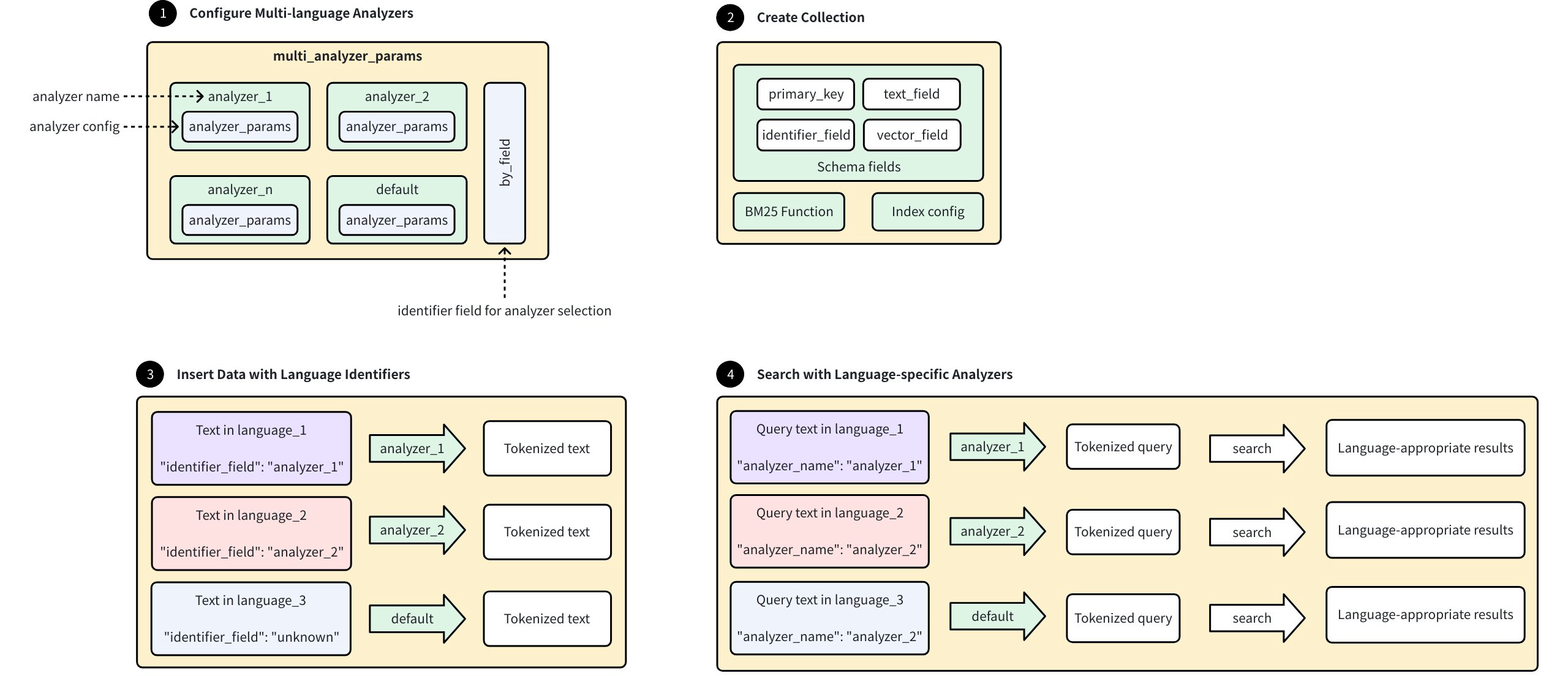
- Configure Multi-language Analyzers:
- Set up multiple language-specific analyzers using the format:
<analyzer_name>: <analyzer_config>, where eachanalyzer_configfollows standardanalyzer_paramsconfiguration as described in Analyzer Overview. - Define a special identifier field that will determine analyzer selection for each document.
- Configure a
defaultanalyzer for handling unknown languages.
- Set up multiple language-specific analyzers using the format:
- Create Collection:
- Define schema with essential fields:
- primary_key: Unique document identifier.
- text_field: Stores original text content.
- identifier_field: Indicates which analyzer to use for each document.
- vector_field: Stores sparse embeddings to be generated by the BM25 function.
- Configure BM25 function and indexing parameters.
- Define schema with essential fields:
- Insert Data with Language Identifiers:
- Add documents containing text in various languages, where each document includes an identifier value specifying which analyzer to use.
- Milvus selects the appropriate analyzer based on the identifier field, and documents with unknown identifiers use the
defaultanalyzer.
- Search with Language-Specific Analyers:
- Provide query text with an analyzer name specified, and Milvus processes the query using the specified analyzer.
- Tokenization occurs according to language-specific rules, and search returns language-appropriate results based on similarity.
# Step 1: Configure multi_analyzer_params
The multi_analyzer_params is a single JSON object that determines how Milvus selects the appropriate analyzer for each entity:
multi_analyzer_params = {
# Define language-specific analyzers
# Each analyzer follows this format: <analyzer_name>: <analyzer_params>
"analyzers": {
"english": {"type": "english"}, # English-optimized analyzer
"chinese": {"type": "chinese"}, # Chinese-optimized analyzer
"default": {"tokenizer": "icu"}, # Required fallback analyzer
},
"by_field": "language", # Field determining analyzer selection
"alias": {
"cn": "chinese", # Use "cn" as shorthand for Chinese
"en": "english" # Use "en" as shorthand for English
}
}
2
3
4
5
6
7
8
9
10
11
12
13
14
| Parameter | Required? | Description | Rules |
|---|---|---|---|
analyzers | Yes | Lists every language-specific analyzer that Milvus can use to process text. Each analyzer in analyzers follows this format <analyzer_name>: <analyzer_params> | 1. Define each analyzer with the standard analyzer_params syntax (see Analyzer Overview). 2. Add an entry whose key is default; Milvus falls back to this analyzer whenever the value stored in by_field does not match any other analyzer name. |
by_field | Yes | Name of the field that stores, for every document, the language (that is, the analyzer name) Milvus should apply. | 1. Must be a VARCHAR field defined in the collection. 2. The value in every row must exactly match one of the analyzer names (or aliases) listed in analyzers. 3. If a row's value is missing or not found, Milvus automatically applies the default analyzer. |
alias | No | Creates shortcuts or alternative names for your analyzers, making them easier to reference in your code. Each analyzer can have one or more aliases. | Each alias must map to an existing analyzer key. |
# Step 2: Create collection
Creating a collection with multi-language support requires configuring specific fields and indexes:
# Add fields
In this step, define the collection schema with four essential fields:
- Primary Key Field (
id): A unique identifier for each entity in the collection. Settingauto_id=Trueenables Milvus to automatically generate these IDs. - Language Indicator Field (
language): This VARCHAR field coreesponds to theby_fieldspecified in yourmulti_analyzer_params. It stores the language identifier for each entity, which tells Milvus which analyzer to use. - Text Content Field (
text): This VARCHAR field stores the actual text data you want to analyze and search. Settingenable_analyzer=Trueis crucial as it activates text analysis capabilities for this field. Themulti_analyzer_paramsconfiguration is attached directly to this field, establishing the connection between your text data and language-specific analyzers. - Vector Field (
sparse): This field will store the sparse vectors generated by the BM25 function. These vectors represent the analyzable form of your text data and are what Milvus actually searches.
# Import required modules
from pymilvus import MilvusClient, DataType, Function, FunctionType
# Initialize client
client = MilvusClient(
uri="http://localhost:19530",
)
# Initialize a new schema
schema = client.create_schema()
# Step 2.1: Add a primary key field for unique document identification
schema.add_field(
field_name="id", # Field name
datatype=DataType.INT64, # Integer data type
is_primary=True, # Designate as primary key
auto_id=True # Auto-generate IDs (recommended)
)
# Step 2.2: Add language identifier field
# This MUST match the "by_field" value in language_analyzer_config
schema.add_field(
field_name="language", # Field name
datatype=DataType.VARCHAR, # String data type
max_length=255 # Maximum length (adjust as needed)
)
# Step 2.3: Add text content field with multi-language analysis capability
schema.add_field(
field_name="text", # Field name
datatype=DataType.VARCHAR, # String data type
max_length=8192, # Maximum length (adjust based on expected text size)
enable_analyzer=True, # Enable text analysis
multi_analyzer_params=multi_analyzer_params # Connect with our language analyzers
)
# Step 2.4: Add sparse vector field to store the BM25 output
schema.add_field(
field_name="sparse", # Field name
datatype=DataType.SPARSE_FLOAT_VECTOR # Sparse vector data type
)
2
3
4
5
6
7
8
9
10
11
12
13
14
15
16
17
18
19
20
21
22
23
24
25
26
27
28
29
30
31
32
33
34
35
36
37
38
39
40
41
# Define BM25 function
Define a BM25 function to generate sparse vector representations from your raw text data:
# Create the BM25 function
bm25_function = Function(
name="text_to_vector", # Descriptive function name
function_type=FunctionType.BM25, # Use BM25 algorithm
input_field_names=["text"], # Process text from this field
output_field_name=["sparse"] # Store vectors in this field
)
# Add the function to our schema
schema.add_function(bm25_function)
2
3
4
5
6
7
8
9
10
This function automatically applies the appropriate analyzer to each text entry based on its language identifier. For more information on BM25-based text retrieval, refer to Full Text Search.
# Configure index params
To allow efficient searching, create an index on the sparse vector field:
# Configure index parameters
index_params = client.prepare_index_params()
# Add index for sparse vector field
index_params.add_index(
field_name="sparse", # Field to index (our vector field)
index_type="AUTOINDEX", # Let Milvus choose optimal index type
metric_type="BM25" # Must be BM25 for this feature
)
2
3
4
5
6
7
8
9
The index improves search performance by organizing sparse vectors for efficient BM25 similarity calculations.
# Create the collection
This final creation step brings together all your previous configurations:
collection_name="multilang_demo": names your collection for future reference.schema=schema: applies the field structure and function you defined.index_params=index_params: implements the indexing strategy for efficient searches.
# Create collection
COLLECTION_NAME = "multilingual_documents"
# Check if collection already exists
if client.has_collection(COLLECTION_NAME):
client.drop_collection(COLLECTION_NAME) # Remove it for this example
print(f"Dropped existing collection: {COLLECTION_NAME}")
# Create the collection
client.create_collection(
collection_name=COLLECTION_NAME, # Collection name
schema=schema, # Our multilingual schema
index_params=index_params # Our search index configuration
)
2
3
4
5
6
7
8
9
10
11
12
13
14
At this point, Milvus creates an empty collection with multi-language analyzer support, ready to receive data.
# Step 3: Insert example data
When adding documents to your multi-language collection, each must include both text content and a language identifier:
documents = [
# English documents
{
"text": "Artificial intelligence is transforming technology",
"language": "english", # Using full language name
},
{
"text": "Machine learning models require large datasets",
"language": "en", # Using our defined alias
},
# Chinese documents
{
"text": "人工智能正在改变技术领域",
"language": "chinese", # Using full language name
},
{
"text": "机器学习模型需要大型数据集",
"language": "cn", # Using our defined alias
},
]
result = client.insert(COLLECTION_NAME, documents)
inserted = result["insert_count"]
print(f"Successfully inserted {inserted} documents")
print("Documents by language: 2 English, 2 Chinese")
# Expected output:
# Successfully inserted 4 documents
# Documents by language: 2 English, 2 Chinese
2
3
4
5
6
7
8
9
10
11
12
13
14
15
16
17
18
19
20
21
22
23
24
25
26
27
28
29
30
During insertion, Milvus:
- Reads each document's
languagefield - Applies the corresponding analyzer to the
textfield - Generates a sparse vector representation via the BM25 function
- Stores both the original text and the generated sparse vector
NOTE
You don't need to provide the sparse vector directly; the BM25 function generates it automatically based on your text and the specified analyzer.
# Step 4: Perform search operations
# Use English analyzer
When searching with multi-language analyzers, search_params contains crucial configuration:
metric_type="BM25": must match your index configuration.analyzer_name="english": specifies which analyzer to apply to your query text. This is independent of the analyzers used on stored documents.params={"drop_ratio_search": "0"}: Controls BM25-specific behavior; here, it retains all terms in the search. For more information, refer to Sparse Vector.
search_params = {
"metric_type": "BM25", # Must match index configuration
"analyzer_name": "english", # Analyzer that matches the query language
"drop_ratio_search": "0", # Keep all terms in search (tweak as needed)
}
english_results = client.search(
collection_name=COLLECTION_NAME, # Collection to search
data=["artificial intelligence"], # Query text
anns_field="sparse", # Field to search against
search_params=search_params, # Search configuration
limit=3, # Max results to return
output_fields=["text", "language"], # Fields to include in the output
consistency_level="Bounded", # Data‑consistency guarantee
)
print("\n=== English Search Results ===")
for i, hit in enumerate(english_results[0]):
print(f"{i+1}. [{hit.score:.4f}] {hit.entity.get('text')} "
f"(Language: {hit.entity.get('language')})")
# Expected output:
# === English Search Results ===
# 1. [2.7881] Artificial intelligence is transforming technology (Language: english)
2
3
4
5
6
7
8
9
10
11
12
13
14
15
16
17
18
19
20
21
22
23
24
# Use Chinese analyzer
This example demonstrates switching to the Chinese analyzer (using its alias "cn") for different query text. All other parameters remain the same, but now the query text is processed using Chinese-specific tokenization rules.
search_params["analyzer_name"] = "cn"
chinese_results = client.search(
collection_name=COLLECTION_NAME, # Collection to search
data=["人工智能"], # Query text
anns_field="sparse", # Field to search against
search_params=search_params, # Search configuration
limit=3, # Max results to return
output_fields=["text", "language"], # Fields to include in the output
consistency_level="Bounded", # Data‑consistency guarantee
)
print("\n=== Chinese Search Results ===")
for i, hit in enumerate(chinese_results[0]):
print(f"{i+1}. [{hit.score:.4f}] {hit.entity.get('text')} "
f"(Language: {hit.entity.get('language')})")
# Expected output:
# === Chinese Search Results ===
# 1. [3.3814] 人工智能正在改变技术领域 (Language: chinese)
2
3
4
5
6
7
8
9
10
11
12
13
14
15
16
17
18
19
20
# Choose the Right Analyzer for Your Use Case
NOTE
This guide focuses on practial decision-making for analyzer selection. For technical details about analyzer components and how to add analyzer parameters, refer to Analyzer Overview.
# Understand analyzers in 2 minutes
In Milvus, an analyzer processes the text stored in this field to make it searchable for features like full text search(BM25), phrase match, or text match. Think of it as a text processor that transforms your raw content into searchable tokens.
An analyzer works in a simple, two-stage pipline:

- Tokenization(required): This initial stage applies a tokenizer to break a continuous string of text into discrete, meaningful units called tokens. The tokenization method can vary significantly depending on the language and content type.
- Token filtering(optional): After tokenization, filters are applied to modify, remove, or refine the tokens. These operations can include converting all tokens to lowercase, removing common meaningless words (such as stopwords), or reducing words to their root form (stemming).
Example:
Input: "Hello World!"
1. Tokenization → ["Hello", "World", "!"]
2. Lowercase & Punctuation Filtering → ["hello", "world"]
2
3
# Why the choice of analyzer matters
Choosing the wrong analyzer can make relevant documents unsearchable or return irrelevant results.
The following table summarizes common problems caused by improper analyzer selection and provides actionable solutions for diagnosing search issues.
| Problem | Symptom | Example (Input & Output) | Cause (Bad Analyzer) | Solution (Good Analyzer) |
|---|---|---|---|---|
| Over-tokenization | Text queries for technical terms, identifiers, or URLs fail to find relevant documents. | "user_id" -> ['user', 'id'], "C++" -> ['c'] | standard analyzer | Use a whitespace tokenizer; combine with an alphanumonly filter. |
| Under-tokenization | Search for a component of a multi-word phrase fails to return documents containing the full phrase. | "state-of-the-art" -> ['state'] | ||
| Language Mismatches | Search results for a specific language are nonsensical or nonexistent. | Chinese text: "机器学习" -> ['机器学习'] (one token) | english analyzer | Use a language specific analyzer, such as chinese. |
# First question: Do you need to choosen an analyzer?
For many use cases, you don't need to do anything special. Let's determine if you're one of them.
# Default behavior: standard analyzer
If you don't specify an analyzer when using text retrieval features like full text search, Milvus automatically uses the standard analyzer.
The standard analyzer:
- Splits text on spaces and punctuation.
- Converts all tokens to lowercase.
- Removes a built-in set of common English stop words and most punctuation.
Example transformation:
Input: "The Milvus vector database is built for scale!"
Output: ['the', 'milvus', 'vector', 'database', 'is', 'built', 'scale']
2
# Decision criteria: A quick check
Use this table to quickly determine if the default standard analyzer meets your needs. If it doesn't, you'll need to choose a different path.
| Your Content | Standard Analyzer OK? | Why | What You Need |
|---|---|---|---|
| English blog posts | ✅Yes | Default behavior is sufficient | Use the default (no configuration needed). |
| Chinese documents | ❌No | Chinese words have no spaces and will be treated as one token. | Use a built-in chinese analyzer. |
| Technical documentation | ❌No | Punctuation is stripped from terms like C++ | Create a custom analyzer with a whitespace tokenizer and an alphanumonly filter. |
| Space-separated languages such as French/Spanish text | ⚠️Maybe | Accented characters(café vs. cafe) may not match. | A custom analyzer with the asciifolding is recommended for better results. |
| Multilingual or unkown languages | ❌No | The standard analyzer lacks the language-specific logic needed to handle different character sets and tokenization rules. | Use a custom analyzer with the icu tokenizer for unicode-aware tokenization. Alternatively, consider configuring multi-language analyzers or a language identifier for more precise handling of multilingual content. |
If the default standard analyzer cannot meet your requirements, you need to implement a different one. You have two paths:
# Path A: Use built-in analyzers
Built-in analyzers are pre-configured solutions for common languages. They are the easiest way to get started when the default standard analyzer isn't a perfect fit.
# Available built-in analyzers
| Analyzer | Language Support | Components | Notes |
|---|---|---|---|
standard | Most space-separated languages (English, French, German, Spanish, etc.) | Tokenizer: standard, Filters: lowercase | General-purpose analyzer for initial text processing. For monolingual scenarios, language-specific analyzers (like english) provide better performance. |
english | Dedicated to English, which applies stemming and stop word removal for better English semantic matching | Tokenizer: standard, Filters: lowercase, stemmer, stop | Recommended for English-only content over standard. |
chinese | Chinese | Tokenizer: jieba, Filters: cnalphanumonly | Currently uses Simplified Chinese dictionary by default. |
# Implementation example
To use a built-in analyzer, simply specify its type in the analyzer_params when defining your field schema.
# Using built-in English analyzer
analyzer_params = {
"type": "english"
}
# Applying analyzer config to target VARCHAR field in your collection schema
schema.add_field(
field_name='text',
datatype=DataType.VARCHAR,
max_length=200,
enable_analyzer=True,
analyzer_params=analyzer_params,
)
2
3
4
5
6
7
8
9
10
11
12
13
NOTE
For detail usage, refer to Full Text Search, Text Match, or Phrase Match.
# Path B: Create a custom analyzer
When built-in options don't meet your needs, you can create a custom analyzer by combining a tokenizer with a set of filters. This gives you full control over the text processing pipeline.
# Step 1: Select the tokenizer based on language
Choose your tokenizer based on your content's primary language:
Western languages: For space-separated languages, you have these options:
| Tokenizer | How it Works | Best For | Examples |
|---|---|---|---|
standard | Splits text based on spaces and punctuation marks | General text, mixed punctuation | Input: "Hello, world! Visit example.com", Output: ['Hello', 'world', 'Visit', 'example', 'com'] |
whitespace | Splits only on whitespace characters | Pre-processed content, user formatted text | Input: "user_id = get_user_data()", Output: ['user_id', '=', 'get_user_data()'] |
East Asian languages: Dictionary-based languages require specialized tokenizers for proper word segmentation:
Chinese:
| Tokenizer | How It Works | Best For | Examples |
|---|---|---|---|
jieba | Chinese dictionary-based segmentation with intelligent algorithm | Recommended for Chinese content - combines dictionary with intelligent algorithms, specifically designed for Chinese. | Input: "机器学习时人工智能的一个分支", Output: ['机器', '学习', '是', '人工', '智能', '人工智能', '的', '一个', '分支'] |
lindera | Pure dictionary-based morphological analysis with Chinese dictionary (cc-cedict) | Compared to jieba, processes Chinese text in a more generic manner | Input: "机器学习算法", Output: ["机器", "学习", "算法"] |
Japanese and Korean:
|Language|Tokenizer|How It Works|Best For|Examples|
|:--|:--|:--|:--|
|Japanese|lindera|ipadic(general purpose), ipadic-neologd(modern terms), unidic(academic)|Morphological analysis with proper noun handling|Input: "東京都渋谷区", Output: ["東京", "都", "渋谷", "区"]|
|Korean|lindera|ko-dic|Korean morphological analysis|Input: "안녕하세요", Output: ["안녕", "하", "세요"]|
Multilingual or unknown languages: For content where languages are unpredictable or mixed within documents:
| Tokenizer | How It Works | Best For | Examples |
|---|---|---|---|
icu | Unicode-aware tokenization (International Components for Unicode) | Mixed scripts, unkown languages, or when simple tokenization is sufficient. | Input: "Hello 世界 مرحبا", Output: ['Hello', ' ', '世界', ' ', 'مرحبا'] |
When to use icu:
- Mixed languages where language identification is impractical.
- You don't want the overhead of multi-language analyzers or the language identifier.
- Content has a primary language with occasional foreign words that contribute little to the overall meaning (e.g., English text with sporadic brand names or technical terms in Japanese or French).
Alternative approaches: For more precise handling of multilingual content, consider using multi-language analyzers or the language identifier. For details, refer to Multi-language Analyzers or Language Identifier.
# Step 2: Add filters for precision
After selecting your tokenizer, apply filters based on your specific search requirements and content characteristics.
Commonly used filters: These filters are essential for most space-separated language configurations (English, French, German, Spanish, etc.) and significantly improve search quality:
| Filter | How It Works | When to Use | Examples |
|---|---|---|---|
lowercase | Convert all tokens to lowercase | Universal-applies to all languages with case distinctions | Input: ["Applie", "iPhone"], Output: [['apple'], ['iphone']] |
stemmer | Reduce words to their root form | Languages with word inflections (English, French, German, etc.) | For English: Input: ["running", "runs", "ran"], Output: [['run'], ['run'], ['ran']] |
stop | Remove common meaningless words | Most languages - particularly effective for space-separated languages | Input: ["the", "quick", "brown", "fox"], Output: [[], ['quick'], ['brown'], ['fox']] |
NOTE
For East Asian languages (Chinese, Japanese, Korean, etc.), focus on language-specific filters instead. These languages typically use different approaches for text processing and may not benefit significantly from stemming.
Text normalization filters: These filters standardize text variations to improve matching consistency:
| Filter | How It Works | When to Use | Examples |
|---|---|---|---|
asciifolding | Convert accented characters to ASCII equivalents | International content, user-generated content | Input: ["café", "naïve", "résumé"], Output: [['cafe'], ['naive'], ['resume']] |
Token filtering: Control which tokens are preserved based on character content or length:
| Filter | How It Works | When to Use | Examples |
|---|---|---|---|
removepunct | Remove standalone punctuation tokens | Clean output from jieba, lindera, icu tokenizers, which will return punctuations as single tokens | Input: ["Hello", "!", "world"], Output: [['Hello'], ['world']] |
alphanumonly | Keep only letters and numbers | Techinical content, clean text processing | Input: ["user123", "test@email.com"], Output: [['user123'], ['test', 'email', 'com']] |
length | Remove tokens outside specified length range | Filter noise (excessively long tokens) | Input: ["a", "very", "extraordinarily"], Output: [['a'], ['very'], []] (if max=10) |
regex | Custom patern based filtering | Domain-specific token requirements | Input: ["test123", "prod456"], Output: [[], ['prod456']] (if expr="^prod") |
Language-specific filters: These filters handle specific language characteristics:
| Filter | Language | How It Works | Example |
|---|---|---|---|
decompounder | German | Splits compound words into searchable components | Input: ["dampfschifffahrt"], Output: [['dampf', 'schiff', 'fahrt']] |
| cnalphanumonly | Chinese | Keeps Chinese characters + alphanumeric | Input: ["Hello", "世界", "123", "!@#"], Output: [['Hello'], ['世界'], ['123'], []] |
cncharonly | Chinese | Keeps only Chinese characters | Input: ["Hello", "世界", "123"], Output: [[], ['世界'], []] |
# Step 3: Combine and implement
To create your custom analyzer, you define the tokenizer and a list of filters in the analyzer_params dictionary. The filters are applied in the order they are listed.
# Example: A custom analyzer for technical content
analyzer_params = {
"tokenizer": "whitespace",
"filter": ["lowercase", "alphanumonly"]
}
# Applying analyzer config to target VARCHAR field in your collection schema
schema.add_field(
field_name='text',
datatype=DataType.VARCHAR,
max_length=200,
enable_analyzer=True,
analyzer_params=analyzer_params,
)
2
3
4
5
6
7
8
9
10
11
12
13
14
# Final: Test with run_analyzer
Always validate your configuration before applying to a collection:
# Sample text to analyze
sample_text = "The Milvus vector database is built for scale!"
# Run analyzer with the defined configuration
result = client.run_analyzer(sample_text, analyzer_params)
print("Analyzer output:", result)
2
3
4
5
6
Common issues to check:
- Over-tokenization: Technical terms being split incorrectly
- Under-tokenization: Phrases not being separated properly
- Missing tokens: Important terms being filtered out
For detailed usage, refer to run_analyzer.
# Recommended configurations by use case
This section provides recommended tokenizer and filter configurations for common use cases when working with analyzers in Milvus. Choose the combination that best matches your content type and search requirements.
NOTE
Before applying an analyzer to your collection, we recommend you use run_analyzer to test and validate text analysis performance.
# Langauges with accent marks (French, Spanish, German, etc.)
Use a standard tokenizer with lowercase conversion, language-specific stemming, and stopword removal. This configuration also works for other European languages by modifying the language and stop_words parameters.
# French exmaple
analyzer_params = {
"tokenizer": "standard",
"filter": [
"lowercase",
"asciifolding", # Handle accent marks
{
"type": "stemmer",
"language": "french"
},
{
"type": "stop",
"stop_words": ["_french_"]
}
]
}
# For other languages, modify the language parameter:
# "language": "spanish" for Spanish
# "language": "german" for German
# "stop_words": ["_spanish_"] or ["_german_"] accordingly
2
3
4
5
6
7
8
9
10
11
12
13
14
15
16
17
18
19
20
21
# English content
For English text processing with comprehensive filtering. You can also use the built-in english analyzer:
analyzer_params = {
"tokenizer": "standard",
"filter": [
"lowercase",
{
"type": "stemmer",
"language": "english"
},
{
"type": "stop",
"stop_words": ["_english_"]
}
]
}
# Equivalent built-in shortcut:
analyzer_params = {
"type": "english"
}
2
3
4
5
6
7
8
9
10
11
12
13
14
15
16
17
18
19
# Chinese content
Use the jieba tokenizer and apply a character filter to retain only Chinese characters, Latin letters, and digits.
analyzer_params = {
"tokenizer": "jieba",
"filter": ["cnalphanumonly"]
}
# Equivalent built-in shortcut:
analyzer_params = {
"type": "chinese"
}
2
3
4
5
6
7
8
9
NOTE
For Simplified Chinese, cnalphanumonly removes all tokens except Chinese characters, alphanumeric text, and digits. This prevents punctuation from affecting search quality.
# Japanese content
Use the lindera tokenizer with Japanese dictionary and filters to clean punctuation and control token length:
analyzer_params = {
"tokenizer": {
"type": "lindera",
"dict": "ipadic" # Options: ipadic, ipadic-neologd, unidic
},
"filter": [
"removepunct", # Remove standalone punctuation
{
"type": "length",
"min": 1,
"max": 20
}
]
}
2
3
4
5
6
7
8
9
10
11
12
13
14
15
# Korean content
Similar to Japanese, using lindera tokenizer with Korean dictionary:
analyzer_params = {
"tokenizer": {
"type": "lindera",
"dict": "ko-dic"
},
"filter": [
"removepunct",
{
"type": "length",
"min": 1,
"max": 20
}
]
}
2
3
4
5
6
7
8
9
10
11
12
13
14
# Mixed or multilingual content
When working with content that spans multiple languages or uses scripts unpredictably, start with the icu analyzer. This Unicode-aware analyzer handles mixed scripts and symbols effectively.
Basic multilingual configuration (no stemming):
analyzer_params = {
"tokenizer": "icu",
"filter": ["lowercase", "asciifolding"]
}
2
3
4
Advanced multilingual processing: For better control over token behavior across different languages:
- Use a multi-language analyzer configuration. For details, refer to Multi-language Analyzers
- Implement a language identifier on your content. For details, refer to Language Identifier.
# Integrate with text retrieval features
After selecting your analyzer, you can integrate it with text retrieval features provided by Milvus.
- Full text search: Analyzers directly impact BM25-based full text search through sparse vector generaion. Use the same analyzer for both indexing and querying to ensure consistent tokenization. Language-specific analyzers generally provide better BM25 scoring than generic ones. For implementation details, refer to Full Text Search.
- Text Match: Text match operations perform exact token matching between queries and indexed content based on your analyzer output. For implementation details, refer to Text Match.
- Phrase match: Phrase match requires consistent tokenization across multi-word expressions to maintain phrase boundaries and meaning. For implementation details, refer to Phrase Match.
# Alter Collection Field
You can alter the properties of a collection field to change column constraints or enforce stricter data integrity rules.
NOTE
- Each collection consists of only one primary field. Once set during collection creation, you cannot change the primary field or alter its properties.
- Each collection can have only one partition key. Once set during collection creation, you cannot change the partition key.
# Alter VarChar field
A VarChar field has a property named max_length, which constrains the maximum number of characters the field values can contain. You can change the max_length property.
The following example assumes the collection has a VarChar field named varchar and sets its max_length property.
from pymilvus import MilvusClient
client = MilvusClient(
uri="http://localhost:19530",
token="root:Milvus"
)
client.alter_collection_field(
collection_name="my_collection",
field_name="varchar",
field_params={
"max_length": 1024
}
)
2
3
4
5
6
7
8
9
10
11
12
13
14
# Alter ARRAY field
An array field has two properties, namely element_type and max_capacity. The former determines the data type of the elements in an array, while the latter constrains the maximum number of elements in the array. You can change the max_capacity property only.
The following example assumes the collection has an array field named array and sets its max_capacity property.
client.alter_collection_field(
collection_name="my_collection",
field_name="array",
field_params={
"max_capacity": 64
}
)
2
3
4
5
6
7
# Alter field-level mmap settings
Memory mapping (Mmap) enables direct memory access to large files on disk, allowing Milvus to store indexes and data in both memory and hard drives. This approach helps optimize data placement policy based on access frequency, expanding storage capacity for collections without impacting search performance.
The following example assumes the collection has a field named doc_chunk and sets its mmap_enabled property.
client.alter_collection_field(
collection_name="my_collection",
field_name="doc_chunk",
field_params={"mmap.enabled": True}
)
2
3
4
5
# Add Fields to an Existing Collection
Milvus allows you to dynamically add new fields to existing collections, making it easy to evolve your data schema as your application needs change. This guide shows you how to add fields in different scenarios using partical examples.
# Considerations
Before adding fields to your collection, keep these important points in mind:
- You can add scalar fields (
INT64,VARCHAR,FLOAT,DOUBLE, etc.), Vector fields canot be added to existing collections. - New fields must be nullable (nullable=True) to accommodate existing entities that don't have values for the new field.
- Adding fields to loaded collections increases memory usage.
- There's a maximum limit on total fields per collection. For details, refer to Milvus Limits.
- Field names must be unique among static fields.
- You cannot add a
$metafield to enable dynamic field functionality for collections that weren't originally created withenable_dynamic_field=True
# Prerequisites
This guide assumes you have:
- A running Milvus instance
- Milvus SDK installed
- An existing collection
NOTE
Refer to our Create Collection for collection and basic operations.
# Basic usage
from pymilvus import MilvusClient, DataType
# Connect to your Milvus server
client = MilvusClient(
uri="http://localhost:19530" # Replace with your Milvus server URI
)
2
3
4
5
6
# Scenario 1: Quickly add nullable fields
The simplest way to extend your collection is by adding nullable fields. This is perfect when you need to quickly add new attributes to your data.
# Add a nullable field to an existing collection
# This operation:
# - Returns almost immediately (non-blocking)
# - Makes the field available for use with minimal delay
# - Sets NULL for all existing entities
client.add_collection_field(
collection_name="product_catalog",
field_name="created_timestamp", # Name of the new field to add
data_type=DataType.INT64, # Data type must be a scalar type
nullable=True # Must be True for add fields
# Allows NULL values for existing entities
)
2
3
4
5
6
7
8
9
10
11
12
# What to expect
- Existing entities will have NULL for the new field
- New entities can have either NULL or actual values
- Field availability occurs almost immediately with minimal delay due to internal schema synchronization
- Queryable immediately after the brief synchronization period
{
'id': 1,
'created_timestamp': None # New field shows NULL for existing entities
}
2
3
4
# Scenario 2: Add fields with default values
When you want existing entities to have a meaningful initial value instead of NULL, specify default values.
# Add a field with default value
# This operation:
# - Sets the default value for all existing entities
# - Makes the field available with minimal delay
# - Maintains data consistency with the default value
client.add_collection_field(
collection_name="product_catalog",
field_name="priority_level", # Name of the new field
data_type=DataType.VARCHAR, # String type field
max_length=20, # Maximum string length
nullable=True, # Required for added fields
default_value="standard" # Value assigned to existing entities
# Also used for new entities if now value provided
)
2
3
4
5
6
7
8
9
10
11
12
13
14
# What to expect
- Existing entities will have the default value (
"standard") for the newly added field - New entities can override the default value or use it if no value is provided
- Field availability occurs almost immediately with minimal delay
- Queryable immediately after the brief synchronization period
# Example query result
{
'id': 1,
'priority_level': 'standard' # Shows default value for existing entities
}
2
3
4
5
# FAQ
# Can I enable dynamic schema functionality by adding a $meta field?
No, you cannot use add_collection_field to add a $meta field to enable dynamic field functionality. Dynamic schema must be enabled when creating the collection by setting enable_dynamic_field=True in the schema.
# ❌ This is NOT supported
client.add_collection_field(
collection_name="existing_collection",
field_name="$meta",
data_type=DataType.JSOn # This operation will fail
)
# ✅ Dynamic field must be enabled during collection creation
client.create_collection(
collection_name="my_collection",
dimension=5,
enable_dynamic_field=True
)
2
3
4
5
6
7
8
9
10
11
12
13
# What happens when I add a field with the same name as a dynamic field key?
When your collection has dynamic field enabled ($meta exists), you can add static fields that have the same name as existing dynamic field keys. The new static field will mask the dynamic field key, but the original dynamic data is preserved.
Example scenario:
# Original collection with dynamic field enabled
# Insert data with dynamic field keys
data = [
{
"id": 1,
"my_vector": [0.1, 0.2, ...]
"extra_info": "this is a dynamic field key", # Dynamic field key as string
"score": 99.5 # ANother dynamic field key
}
]
client.insert(collection_name="product_catalog", data=data)
# Add static field with same name as existing dynamic field key
client.add_collection_field(
collection_name="product_catalog",
field_name="extra_info", # Same name as dynamic field key
data_type=DataType.INT64, # Data type can differ from dynamic field key
nullable=True # Must be True for add fields
)
# Insert new data after adding static field
new_data = [
{
"id": 2,
"my_vector": [0.3, 0.4, ...],
"extra_info": 100, # Now must use INT64 type (static field)
"score": 88.0 # Still a dynamic field key
}
]
client.insert(collection_name="product_catalog", data=new_data)
2
3
4
5
6
7
8
9
10
11
12
13
14
15
16
17
18
19
20
21
22
23
24
25
26
27
28
29
30
What to expect:
- Existing entities will have NULL for the new static field
extra_info - New entities must use the static field's data type (
INT64) - Original dynamic field key values are preserved and accessible via
$metasyntax - The static field masks the dynamic field key in normal queries
Accessing both static and dynamic values:
# 1. Query static field only (dynamic field key is marked)
results = client.query(
collection_name="product_catalog",
filter="id == 1",
output_fields=["extra_info"]
)
# Returns: {"id": 1, "extra_info": None} # NULL for existing entity
# 2. Query both static and original dynamic values
results = client.query(
collection_name="product_catalog",
filter="id == 1",
output_fields=["extra_info", "$meta['extra_info']"]
)
# Returns: {
# "id": 1,
# "extra_info": None, # Static field value (NULL)
# "$meta['extra_info']": "this is a dynamic field key" # Original dynamic value
# }
# 3. Query new entity with static field value
results = client.query(
collection_name="product_catalog",
filter="id == 2",
output_fields=["extra_info"]
)
# Returns: {"id": 2, "extra_info": 100} # Static field value
2
3
4
5
6
7
8
9
10
11
12
13
14
15
16
17
18
19
20
21
22
23
24
25
26
27
# How long does it take for a new field to become avilable?
Added fields become available almost immediately, but there may be a brief delay due to internal schema change broadcasting across the Milvus cluster. This synchronization ensures all nodes are aware of the schema update before processing queries involving the new field.
# Insert & Delete
# Insert Entities
Entities in a collection are data records that share the same set of fields. Field values in every data record form an entity. This page introduces how to insert entities into a collection.
NOTE
If you dynamically add new fields after the collection has been created, and you do not specify values for these fields when inserting entities, Milvus automatically populates them with either defined default values or NULL if defaults are not set. For details, refer to Add Fields to an Existing Collection.
NOTE:
- Fields added after collection creation: If you add new fields to a collection after creation and don't specify values during insertion, Milvus automatically populates them with defined default values or NULL if no defaults are set. For details, refer to Add Fields to an Existing Collection.
- Duplicate handling: The standard
insertoperation does not check for duplicate primary keys. Inserting data with an existing primary key creates a new entity with the same key, leading to data duplication and potential application issues. To update existing entities or avoid duplicates, use theupsertoperation instead. For more information, refer to Upsert Entities.
# Overview
In Milvus, an Entity refers to data records in a Collection that share the same Schema, with the data in each field of a row constituting an Entity. Therefore, the Entities within the same Collection have the same attributes (such as field names, data types, and other constraints).
When inserting an Entity into a Collection, the Entity to be inserted can only be successfully added if it contains all the fields defined in the Schema. The inserted Entity will enter a Partition named _default in the order of insertion. Provided that a certain Partition exists, you can also insert Entities into that Partition by specifying the Partition name in the insertion request.
Milvus also supports dynamic fields to maintain the scalability of the Collection. When the dynamic field is enabled, you can insert fields that are not defined in the Schema into the Collection. These fields and values will be stored as key-value pairs in a reserved field named $meta. For more information about dynamic fields, please refer to Dynamic Field.
# Insert Entities into a Collection
Before inserting data, you need to organize your data into a list of dictionaries according to the Schema, with each dictionary representing an Entity and containing all the fields defined in the Schema. If the Collection has the dynamic field enabled, each dictionary can also include fields that are not defined in the Schema. In this section, you will insert entities into a Collection created in the quick-setup manner. A Collection created in this manner has only two fields, named id and vector. Additionally, this Collection has the dynamic field enabled, so the Entities in the example code include a field called color that is not defined in the Schema.
from pymilvus import MilvusClient
client = MilvusClient(
uri="http://localhost:19530",
token="root:Milvus"
)
data=[
{"id": 0, "vector":
[0.3580376395471989, -0.6023495712049978, 0.18414012509913835, -0.26286205330961354, 0.9029438446296592],
"color": "pink_8682"
},
{"id": 1, "vector":
[0.19886812562848388, 0.06023560599112088, 0.6976963061752597, 0.2614474506242501, 0.838729485096104],
"color": "red_7025"
},
{"id": 2, "vector":
[0.43742130801983836, -0.5597502546264526, 0.6457887650909682, 0.7894058910881185, 0.20785793220625592],
"color": "orange_6781"
},
{"id": 3, "vector":
[0.3172005263489739, 0.9719044792798428, -0.36981146090600725, -0.4860894583077995, 0.95791889146345],
"color": "pink_9298"
},
{"id": 4, "vector":
[0.4452349528804562, -0.8757026943054742, 0.8220779437047674, 0.46406290649483184, 0.30337481143159106],
"color": "red_4794"
},
{"id": 5, "vector":
[0.985825131989184, -0.8144651566660419, 0.6299267002202009, 0.1206906911183383, -0.1446277761879955],
"color": "yellow_4222"
},
{"id": 6, "vector":
[0.8371977790571115, -0.015764369584852833, -0.31062937026679327, -0.562666951622192, -0.8984947637863987],
"color": "red_9392"
},
{"id": 7, "vector":
[-0.33445148015177995, -0.2567135004164067, 0.8987539745369246, 0.9402995886420709, 0.5378064918413052],
"color": "grey_8510"
},
{"id": 8, "vector":
[0.39524717779832685, 0.4000257286739164, -0.5890507376891594, -0.8650502298996872, -0.6140360785406336],
"color": "white_9381"
},
{"id": 9, "vector":
[0.5718280481994695, 0.24070317428066512, -0.3737913482606834, -0.06726932177492717, -0.6980531615588608],
"color": "purple_4976"
}
]
res = client.insert(
collection_name="quick_setup",
data=data
)
print(res)
# Output
# {'insert_count': 10, 'ids': [0, 1, 2, 3, 4, 5, 6, 7, 8, 9]}
2
3
4
5
6
7
8
9
10
11
12
13
14
15
16
17
18
19
20
21
22
23
24
25
26
27
28
29
30
31
32
33
34
35
36
37
38
39
40
41
42
43
44
45
46
47
48
49
50
51
52
53
54
55
56
57
58
59
# Insert Entities into a Partition
You can also insert entities into a specified partition. The following code snippets assume that you have a partition named PartitionA in your collection.
data=[
{"id": 10, "vector":
[0.3580376395471989, -0.6023495712049978, 0.18414012509913835, -0.26286205330961354, 0.9029438446296592],
"color": "pink_8682"
},
{"id": 11, "vector":
[0.19886812562848388, 0.06023560599112088, 0.6976963061752597, 0.2614474506242501, 0.838729485096104],
"color": "red_7025"
},
{"id": 12, "vector":
[0.43742130801983836, -0.5597502546264526, 0.6457887650909682, 0.7894058910881185, 0.20785793220625592],
"color": "orange_6781"
},
{"id": 13, "vector":
[0.3172005263489739, 0.9719044792798428, -0.36981146090600725, -0.4860894583077995, 0.95791889146345],
"color": "pink_9298"
},
{"id": 14, "vector":
[0.4452349528804562, -0.8757026943054742, 0.8220779437047674, 0.46406290649483184, 0.30337481143159106],
"color": "red_4794"
},
{"id": 15, "vector":
[0.985825131989184, -0.8144651566660419, 0.6299267002202009, 0.1206906911183383, -0.1446277761879955],
"color": "yellow_4222"
},
{"id": 16, "vector":
[0.8371977790571115, -0.015764369584852833, -0.31062937026679327, -0.562666951622192, -0.8984947637863987],
"color": "red_9392"
},
{"id": 17, "vector":
[-0.33445148015177995, -0.2567135004164067, 0.8987539745369246, 0.9402995886420709, 0.5378064918413052],
"color": "grey_8510"
},
{"id": 18, "vector":
[0.39524717779832685, 0.4000257286739164, -0.5890507376891594, -0.8650502298996872, -0.6140360785406336],
"color": "white_9381"
},
{"id": 19, "vector":
[0.5718280481994695, 0.24070317428066512, -0.3737913482606834, -0.06726932177492717, -0.6980531615588608],
"color": "purple_4976"
}
]
res = client.insert(
collection_name="quick_setup",
# highlight-next-line
partition_name="partitionA",
data=data
)
print(res)
# Output
# {'insert_count': 10, 'ids': [10, 11, 12, 13, 14, 15, 16, 17, 18, 19]}
2
3
4
5
6
7
8
9
10
11
12
13
14
15
16
17
18
19
20
21
22
23
24
25
26
27
28
29
30
31
32
33
34
35
36
37
38
39
40
41
42
43
44
45
46
47
48
49
50
51
52
53
54
# Upsert Entities
The upsert operation provides a convenient way to insert or update entities in a collection.
# Overview
You can use upsert to either insert a new entity or update an existing one, depending on whether the primary key provided in the upsert request exists in the collection. If the primary key is not found, an insert operation accurs. Otherwise, an update operation will be performed.
An upsert in Milvus works in either override or merge mode.
# Upsert in override mode
An upsert request that works in overide mode combines an insert and a delete. When an upsert request for an existing entity is received, Milvus inserts the data carried in the request payload and deletes the existing entity with the original primary key specified in the data at the same time.
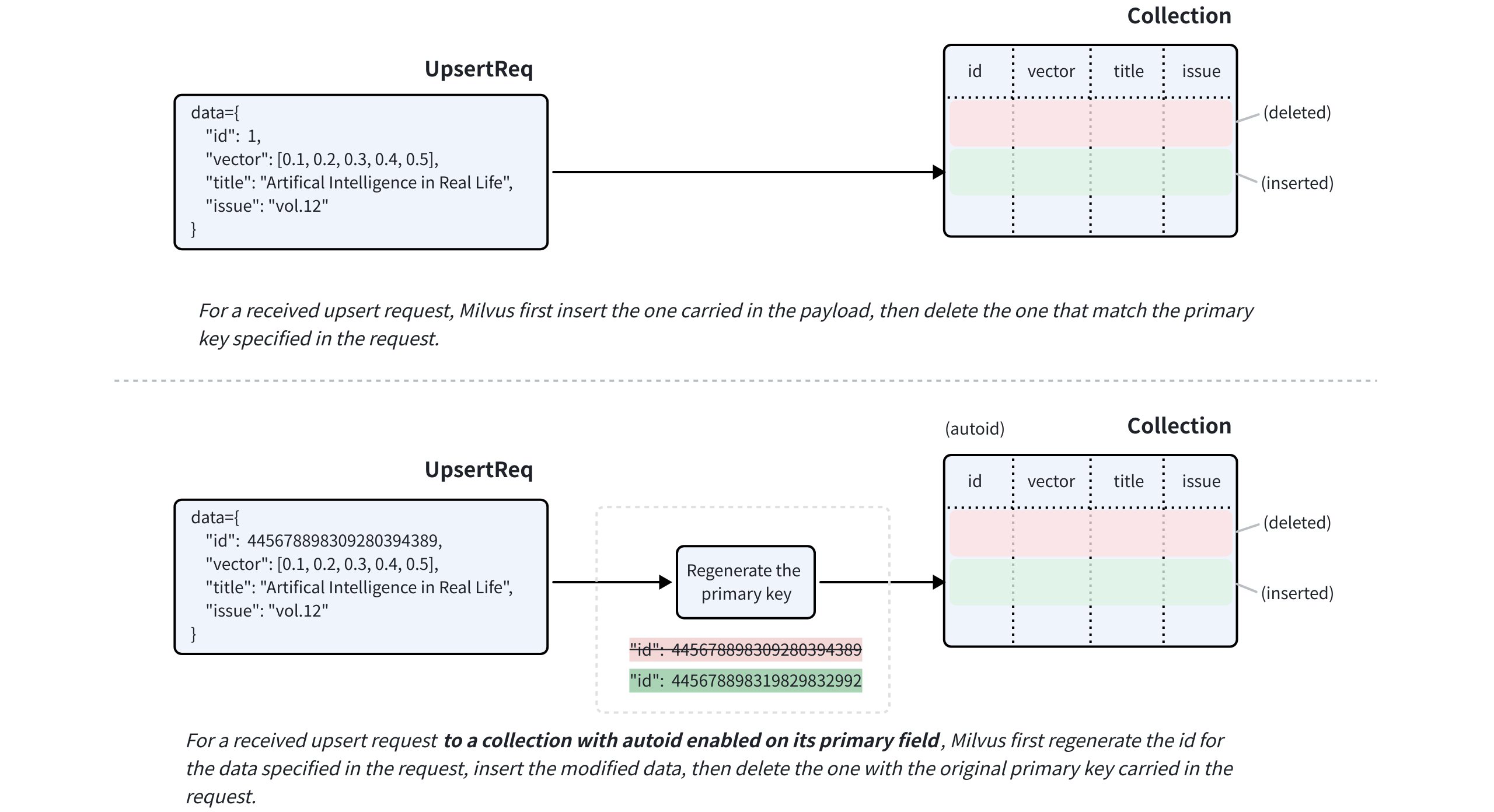
If the target collection has autoid enabled on its primary field, Milvus will generate a new primary key for the data carried in the request payload before inserting it.
For fields with nullable enabled, you can omit them in the upsert request if they do not require any updates.
# Upsert in merge mode
You can also use the partial_update flag to make an upsert request work in merge mode. This allows you to include only the fields that need updating in the request payload.
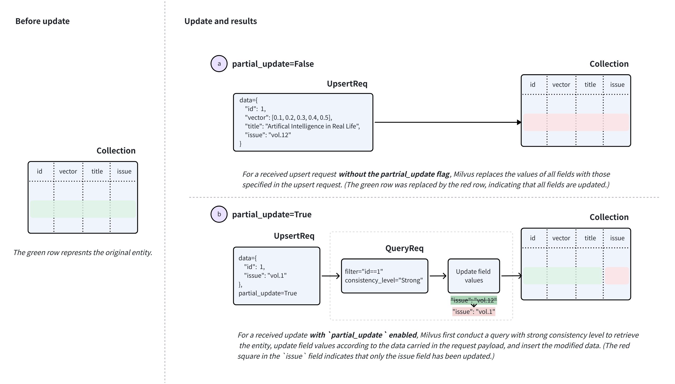
To perform a merge, set partial_update to True in the upsert request along with the primary key and the fields to update with their new values.
Upon receiving such a request, Milvus performs a query with strong consistency to retrieve the entity, updates the field values based on the data in the request, inserts the modified data, and then deletes the existing entity with the original primary key carried in the request.
# Upsert behaviors: special notes
There are several special notes you should consider before using the merge feature. The following cases assume that you have a collection with two scalar fields named title and issue, along with a primary key id and a vector field called vector.
- Upsert fields with
nullableenabled. Suppose that theissuefield can be null. When you upsert these fields, note that:- If you omit the
issuefield in theupsertrequest and disablepartial_update, theissuefield will be updated tonullinstead of retaining its original value. - To preserve the original value of the
issuefield, you need either to enablepartial_updateand omit theissuefield or include theissuefield with its original value in theupsertrequest.
- If you omit the
- Upsert keys in the dynamic field. Suppose that you have enabled the dynamic key in the example collection, and the key-value pairs in the dynamic field of an entity are similar to
{"author": "John", "year": 2020, "tags": ["fiction"]}. When you upsert the entity with keys, such asauthor,year, ortags, or add other keys, note that:- If you upsert with
partial_updatedisabled, the default behavior is to override. It means that the value of the dynamic field will be overriden by all non-schema-defined fields included in the request and their values. For example, if the data included in the request is{"author": "Jane", "genre": "fantasy"}, the key-value pairs in the dynamic field of the target entity will be updated to that. - If you upsert with
partial_updateenabled, the default behavior is to merge. It means that the value of the dynamic field will merge with all non-schema-defined fields included in the request and their values. For example, if the data included in the request is{"author": "John", "year": 2020, "tags": ["fiction"]}, the key-value pairs in the dynamic field of the target entity will become{"author": "Jane", "year": 2020, "tags": ["fiction"], "genre": "fantasy"}after the upsert.
- If you upsert with
- Upsert a JSON field. Suppose that the example collection has a schema-defined JSON field named
extras, and the key-value pairs in this JSON field of an entity are similar to{"author": "John", "year": 2020, "tags": ["fiction"]}. When you upsert theextrasfield of an entity with modified JSON data, note that:- If you upsert with
partial_updatedisabled, the default behavior is to override. It means the value of the JSON field included in the request will override the original value of the target entity's JSON field. For example, if the data included in the request is{extras: {"author": "Jane", "genre": "fantasy"}}, the key-value pairs in theextrasfield of the target entity will be updated to{"author": "Jane", "genre": "fantasy"}. - If you upsert with
partial_updateenabled, the default behavior is to merge. It means the value of the JSON field included in the request will merge with the original value of the target entity's JSON field. For example, if the data included in the request is{extras: {"author": "Jane", "genre": "fantasy"}}, the key-value pairs in theextrasfield of the target entity will become{"author": "Jane", "year": 2020, "tags": ["fiction"], "genre": "fantasy"}after the update.
- If you upsert with
# Limits & Restrictions
Based on the above content, there are several limits and restrictions to follow:
- The
upsertrequest must always include the primary keys of the target entities. - The target collection must be loaded and available for queries.
- All fields specified in the request must exist in the schema of the target collection.
- The values of all fields specified in the request must match the data types defined in the schema.
- For any field derived from another using functions, Milvus will remove the derived field during the upsert to allow recalculation.
# Upsert entities in a collection
In this section, we will upsert entities into a collection named my_collection. This collection has only four fields, named id, vector, title, and issue. The id field is the primary field, while the title and issue fields are scalar fields.
The three entities, if exists in the collection, will be overridden by those included the upsert request.
from pymilvus import MilvusClient
client = MilvusClient(
uri="http://localhost:19530",
token="root:Milvus"
)
data=[
{
"id": 0,
"vector": [-0.619954382375778, 0.4479436794798608, -0.17493894838751745, -0.4248030059917294, -0.8648452746018911],
"title": "Artificial Intelligence in Real Life",
"issue": "vol.12"
}, {
"id": 1,
"vector": [0.4762662251462588, -0.6942502138717026, -0.4490002642657902, -0.628696575798281, 0.9660395877041965],
"title": "Hollow Man",
"issue": "vol.19"
}, {
"id": 2,
"vector": [-0.8864122635045097, 0.9260170474445351, 0.801326976181461, 0.6383943392381306, 0.7563037341572827],
"title": "Treasure Hunt in Missouri",
"issue": "vol.12"
}
]
res = client.upsert(
collection_name='my_collection',
data=data
)
print(res)
# Output
# {'upsert_count': 3}
2
3
4
5
6
7
8
9
10
11
12
13
14
15
16
17
18
19
20
21
22
23
24
25
26
27
28
29
30
31
32
33
34
35
# Upsert entities in a partition
You can also upsert entities into a specified partition. The following code snippets assume that you have a partition named PartitionA in your collection.
The three entities, if exists in the partition, will be overridden by those included in the request.
data=[
{
"id": 10,
"vector": [0.06998888224297328, 0.8582816610326578, -0.9657938677934292, 0.6527905683627726, -0.8668460657158576],
"title": "Layour Design Reference",
"issue": "vol.34"
},
{
"id": 11,
"vector": [0.6060703043917468, -0.3765080534566074, -0.7710758854987239, 0.36993888322346136, 0.5507513364206531],
"title": "Doraemon and His Friends",
"issue": "vol.2"
},
{
"id": 12,
"vector": [-0.9041813104515337, -0.9610546012461163, 0.20033003106083358, 0.11842506351635174, 0.8327356724591011],
"title": "Pikkachu and Pokemon",
"issue": "vol.12"
},
]
res = client.upsert(
collection_name="my_collection",
data=data,
partition_name="partitionA"
)
print(res)
# Output
# {'upsert_count': 3}
2
3
4
5
6
7
8
9
10
11
12
13
14
15
16
17
18
19
20
21
22
23
24
25
26
27
28
29
30
31
# Upsert entities in merge mode
The following code example demonstrates how to upsert entities with partial updates. Provide only the fields needing updates and their new values, along with the explicit partial update flag.
In the following example, the issue field of the entities specified in the upsert request will be updated to the values included in the request.
data=[
{
"id": 3,
"issue": "vol.14"
},
{
"id": 12,
"issue": "vol.7"
}
]
res = client.upsert(
collection_name="my_collection",
data=data,
partial_update=True
)
print(res)
# Output
# {'upsert_count': 2}
2
3
4
5
6
7
8
9
10
11
12
13
14
15
16
17
18
19
20
21
# Delete Entities
You can delete the entities that are no longer needed by filtering conditions or their primary keys.
# Delete Entities by Filtering Conditions
When deleting multiple entities that share some attributes in a batch, you can use filter expressions. The example code below uses the in operator to bulk delete all Entities with their color field set to the values of red and purple. You can also use other operators to construct filter expressions that meet your requirements. For more information about filter expressions, please refer to Filtering Explained.
from pymilvus import MilvusClient
client = MilvusClient(
uri="http://localhost:19530",
token="root:Milvus"
)
res = client.delete(
collection_name="quick_setup",
filter="color in ['red_7025', 'purple_4976']"
)
print(res)
# Output
# {'delete_count': 2}
2
3
4
5
6
7
8
9
10
11
12
13
14
15
16
# Delete Entities by Primary Keys
In most cases, a primary key uniquely identifies an Entity. You can delete Entities by setting their primary keys in the delete request. The example code below demonstrates how to delete two entities with primary keys 18 and 19.
res = client.delete(
collection_name="quick_setup",
ids=[18, 19]
)
print(res)
# Output
# {'delete_count': 2}
2
3
4
5
6
7
8
9
# Delete Entities from Partitions
You can also delete entities sotred in specific partitions. The following code snippets assume that you have a partition named PartitionA in your collection.
res = client.delete(
collection_name="quick_setup",
ids=[18, 19],
partition_name="partitionA"
)
print(res)
# Output
# {'delete_count': 2}
2
3
4
5
6
7
8
9
10
# Indexes
# Index Explained
An index is an additional structure built on top of data. Its internal structure depends on the approximate nearest neighbor search algorithm in use. An index speeds up the search, but incurs additional preprocessing time, space, and RAM during the search. Moreover, using an index typically lowers the recall rate (though the effect is negligible, it still matters). Therefore, this article explains how to minimize the costs of using an index while maximizing the benefits.
# Overview
In Milvus, indexes are specific to fields, and the applicable index types vary according to the data types of the target fields. As a professional vector database, Milvus focuses on enhancing both the performance of vector searches and scalar filtering, which is why it offers various index types.
The following table lists the mapping relationship between field data types and applicable index types.
| Field Data Type | Applicable Index Types |
|---|---|
FLOAT_VECTOR, FLOAT16_VECTOR, BFLOAT16_VECTOR, INT8_VECTOR | FLAT, IVF_FLAT, IVF_SQ8, IVF_PQ, IVF_RABITQ, GPU_IVF_FLAT, GPU_IVF_PQ, HNSW, DISKANN |
BINARY_VECTOR | BIN_FLAT, BIN_IVF_FLAT, MINHASH_LSH |
SPARSE_FLOAT_VECTOR | SPARSE_INVERTED_INDEX |
VARCHAR | INVERTED(Recommended), BITMAP, Trie |
BOOL | BITMAP(Recommended), INVERTED |
INT8, INT16, INT32, INT64 | INVERTED, STL_SORT |
FLOAT, DOUBLE | INVERTED |
ARRAY(elements of the BOOL, INT8/16/32/64, and VARCHAR types) | BITMAP(Recommended) |
ARRAY(elements of the BOOL, INT8/16/32/64, and VARCHAR types) | INVERTED |
JSON | INVERTED |
This article focuses on how to select appropriate vector indexes. For scalar fields, you can always use the recommended index type.
Selecting an appropriate index type for a vector search can significantly impact perfomance and resource usage. When choosing an index type for a vector field, it is essential to consider various factors, including the underlying data structure, memory usage, and performance requirements.
# Vector Index anatomy
As demonstrated in the diagram below, an index type in Milvus consists of three core components, namely data structure, quantization, and refiner. Quantization and refiner are optional, but are widely used because of a significant gains-better-than-costs balance.
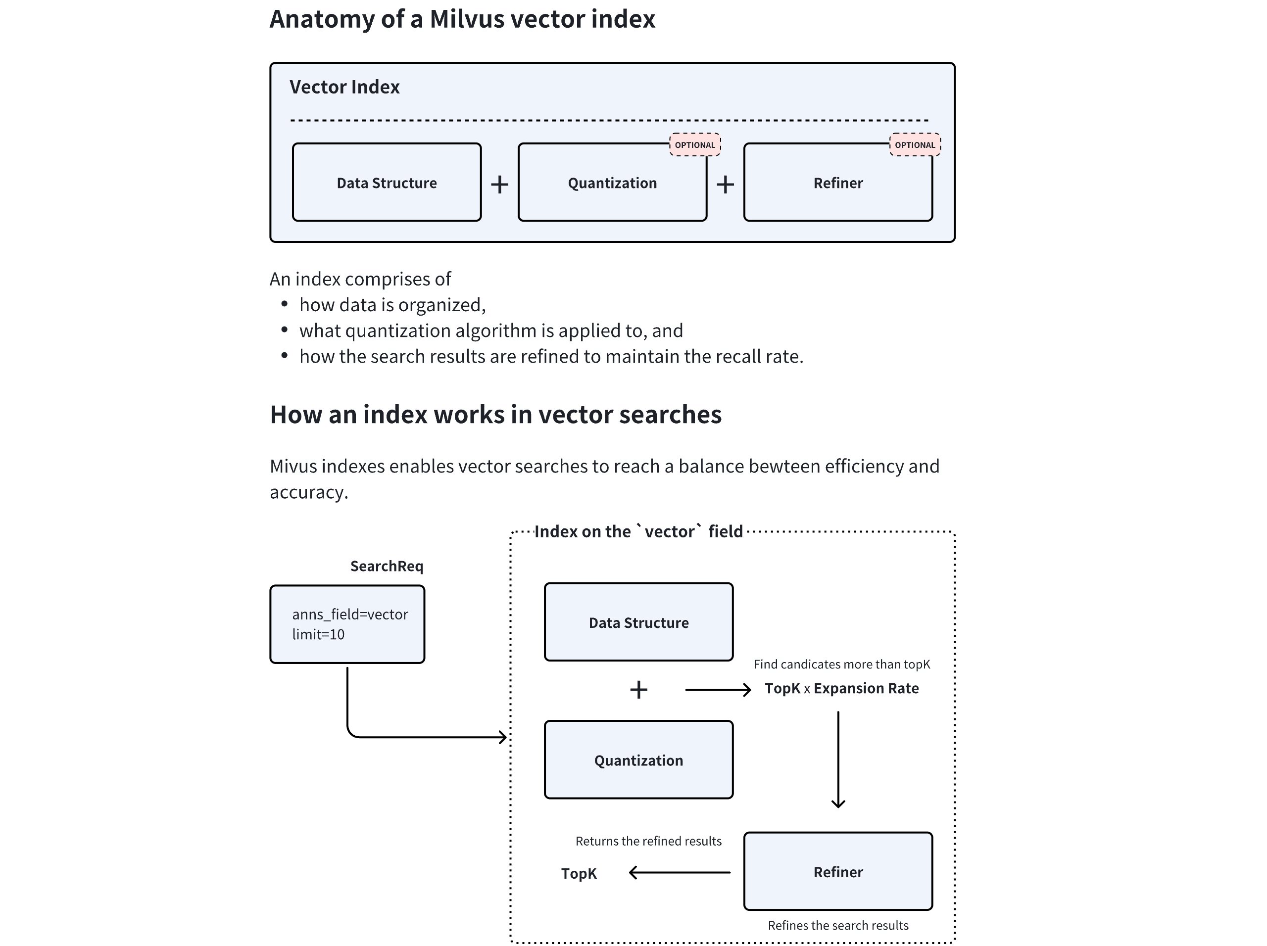
During index creation, Milvus combines the chosen data structure and quantization method to determine an optimal expansion rate. At query time, the system retrieves topK * expansion rate candidate vectors, applies the refiner to recalculate distances with higher precision, and finally returns the most accurate topK results. This hybrid approach balances speed and accuracy by restricting resource-intensive refinement to a filtered subset of candidates.
# Data structure
The data structure forms the foundational layer of the index. Common types include:
- Inverted File(IVF): IVF-series index types allow Milvus to cluster vectors into buckets through centroid-based partitioning. It is generally safe to assume that all vectors in a bucket are likely to be close to the query vector if the bucket centroid is close to the query vector. Based on this premise, Milvus scans only the vector embeddings in those buckets where the centroids are near the query vector, rather than examining the entire dataset. This strategy reduces computational costs while maintaining acceptable accuracy. This type of index data structure is ideal for large-scale datasets requiring fast throughput.
- Graph-based structure: A graph-based data structure for vector search, such as Hierarchical Navigable Small World (HNSW), constructs a layered graph where each vector connects to its nearest. Queries navigate this hierarchy, starting from coarse upper layers and switching through lower layers, enabling efficient logarithmic-time search complexity. This type of index data structure excels in high-dimensional spaces and scenarios demanding low-latency queries.
# Quantization
Quantization reduces memory footprint and computational costs through a coarser representation:
- Scalar Quantization (e.g. SQ8): enables Milvus to compress each vector dimension into a single byte (8-bit), reducing memory usage by 75% compared to 32-bit floats while preserving reasonable accuracy.
- Product Quantization (PQ): enables Milvus to split vectors into subvectors and encode them using codebook-based clustering. This achieves higher compression ratios (e.g., 4-32x) at the cost of marginally reduced recall, making it suitable for memory-constrained environments.
# Refiner
Quantization is inherently lossy. To maintain the recall rate, quantization consistently produces more top-K candidates than necessary, allowing refiners to use higher precision to further slect the top-K results from these candidates, enhancing the recall rate.
For instance, the FP32 refiner operates on the search results candidates returned by quantization by recalculating distances using FP32 precision rather than the quantized values.
This is critical for applications requiring a tradeoff between search efficiency and precision, such as semantic search or recommendation systems, where minor distance variations significantly impact result quality.
# Summary
This tiered architecture -- coarse filtering via data structures, efficient computation through quantization, and precision tuning via refinement -- allows Milvus to optimize the accuracy-performance tradeoff adaptively.
# Performance trade-offs
When evaluating performance, it is crucial to balance build time, query per second(QPS), and recall rate. The general rules are as follows:
- Graph-based index types usually outperform IVF variants in terms of QPS.
- IVF variants particularly fit in the scenarios with a large topK (for example, over 2000).
- PQ typically offers a better recall rate at similar compression rates when compared to SQ, though the letter provides faster performance.
- Using hard drives for part of the index (as in DiskANN) helps manage large datasets, but it also introduces potential IOPS bottlenecks.
# Capacity
Capacity usually involves the raltionship between data size and available RAM. When dealing with capacity, consider the following:
- If a quarter of your raw data fits into memory, consider DiskANN for its stable latency.
- If all your raw data fits into memory, consider memory-based index types and mmap.
- You can use the quantization-applied index types and mmap to trade accuracy for the maximum capacity.
NOTE
Mmap is not always the solution. When most of your data is on disk, DiskANN provides better latency.
# Recall
The recall usually involves the filter ratio, which refers to the data that is filtered out before searches. When dealing with recall, consider the following:
- If the filter ratio is less than 85%, graph-based index types outperform IVF variants.
- If the filter ratio is between 85% and 95%, use IVF variants.
- If the filter ratio is over 98%, use Brute-Force (FLAT) for the most accurate search results.
NOTE
The above items are not always correct. You are advised to tune the recall with different index types to determine which index type works.
# Performance
The performance of a search usually involves the top-K, which refers to the number of records that the search returns. When dealing with performance, consider the following:
- For a search with a small top-K (e.g., 2000) requiring a high recall rate, graph-based index types outperform IVF variants.
- For a search with a great top-K (compared with the total number of vector embeddings), IVF variants are a better choice than graph-based index types.
- For a search with a medium-sized top=K and a high filter ratio, IVF variants are better choices.
# Decision Matrix: Choosing the most appropriate index type
The following table is a decision matrix for you to refer to when choosing an appropriate index type.
| Scenario | Recommended Index | Notes |
|---|---|---|
| Raw data fits in memory | HNSW, IVF + Refinement | Use HNSW for low-k/high recall. |
| Raw data on disk, SSD | DiskANN | Optimal for latency-sensitive queries. |
| Raw data on disk, limited RAM | IVFPQ/SQ + mmap | Balances memory and disk access. |
| High filter ratio (> 95%) | Brute-Force(FLAT) | Avoids index overhead for tiny candidate sets. |
Large k (>= 1% of dataset) | IVF | Cluster pruning reduces computation. |
| Extremely high recall rate (> 99%) | Brute-Force (FLAT) + GPUs | -- |
# Memory usage estimation
NOTE
This section focuses on calculating the memory consumption of a specific index type and includes many technical details. You can skip this section safely if it does not align with your interests.
The memory consumption of an index is influenced by its data structure, compression rate through quantization, and the refiner in use. Generally speaking, graph-based indices typically have a higher memory footprint due to the graph's structure (e.g., HNSW), which usually implies a noticeable per-vector space overhead. In contrast, IVF and its variants are more memory-efficient because less per-vector space overhead applies. However, advanced techniques such as DiskANN allow parts of the index, like the graph or the refiner, to reside on disk, reducing memory load while maintaining performance.
Specifically, the memory usage of an index can be calculated as follows:
# IVF index memory usage
IVF indexes balance memory efficiency with search perfomance by partitioning data into clusters. Below is a breakdown of the memory used by 1 million 128-dimensional vectors indexed using IVF variants.
- Calculate the memory used by centroids. IVF-series index types enable Milvus to cluster vectors into buckets using centroid-based partitioning. Each centroid is included in the index in raw vector embedding. When you divide the vectors into 2000 clusters, the memory usage can be calculated as follows:
2,000 clusters × 128 dimensions × 4 bytes = 1.0 MB
- Calcuate the memory used by cluster assignments. Each vector embedding is assigned to a cluster and stored as integer IDs. For 2000 clusters, a 2-byte integer suffices. The memory usage can be calculated as follows:
1,000,000 vectors × 2 bytes = 2.0 MB
- Calculate the compression caused by quantization. IVF variants typically use PQ and SQ8, and the memory usage can be estimated as follows:
- Using PQ with 8 subquantizers:
1,000,000 vectors × 8 bytes = 8.0 MB - Using SQ8:
1,000,000 vectors × 128 dimensions × 1 byte = 128 MB
- Using PQ with 8 subquantizers:
The following table lists the estimated memory usage with different configurations:
| Configuration | Memory Estimation | Total Memory |
|---|---|---|
| IVF-PQ(no refinement) | 1.0 MB + 2.0 MB + 8.0 MB | 11.0 MB |
| IVF-PQ + 10% raw refinement | 1.0 MB + 2.0 MB + 8.0 MB + 51.2 MB | 62.2 MB |
| IVF-SQ8 (no refinement) | 1.0 MB + 2.0 MB + 128 MB | 131.0 MB |
| IVF-FLAT (full raw vectors) | 1.0 MB + 2.0 MB + 512 MB | 515.0 MB |
- Calculate the refinement overhead. IVF variants often pair with a refiner to re-rank candidates. For a search retrieving the top 10 results with an expansion rate of 5, the refinement overhead can be estimated as follows:
10 (topK) x 5 (expansion rate) = 50 candidates
50 candidates x 128 dimensions x 4 bytes = 25.6 KB
2
# Graph-based index memory usage
Graph-based index types like HNSW require significant memory to store both the graph structure and raw vector embeddings. Below is a detailed breakdown of the memory consumed by 1 million 128-dimensional vectors indexed using the HNSW index type.
- Calculate the memory used by the graph structure. Each vector in HNSW maintains connections to its neighbors. With a graph degree (edges per node) of 32, the memory consumed can be calculated as follows:
1,000,000 vectors × 32 links × 4 bytes (for 32-bit integer storage) = 128 MB
- Calculate the memory used by the raw vector embeddings. The memory consumed by storing uncompressed FP32 vectors can be calculated as follows:
1,000,000 vectors × 128 dimensions × 4 bytes = 512 MB
When you use HNSW to index the 1 million 128-dimensional vector embeddings, the total memory in use would be 128 MB (graph) + 512 MB (vectors) = 640 MB.
- Calculate the compression caused by quantization. Quantization reduces vector size. For example, using PQ with 8 subquantizers (8 bytes per vector) leads to a drastic compression. The memory consumed by the compressed vector embeddings can be calculated as follows:
1,000,000 vectors × 8 bytes = 8 MB
This achieves a 64-times compression rate when compared to the raw vector embeddings, and the total memory used by the HNSWPQ index type would be 128 MB (graph) + 8 MB (compressed vector) = 136 MB.
- Calculate the refinement overhead. Refinement, such as re-ranking with raw vectors, temporarily loads high-precision data into memory. For a search retrieving the top 10 results with an expansion rate of 5, the refinement overhead can be estimated as follows:
10 (topK) x 5 (expansion rate) = 50 candidates
50 candidates x 128 dimensions x 4 bytes = 25.6 KB
2
# Other considerations
While IVF and graph-based indexes optimize memory usage through quantization, memory-mapped files (mmap) and DiskANN address scenarios where datasets exceed available random access memory (RAM).
DiskANN:
DiskANN is a Vamana graph-based index that connects data points for efficient navigation during search while applying PQ to reduce the size of vectors and enable quick approximate distance calculation between vectors.
The Vamana graph is stored on disk, which allows DiskANN to handle large datasets that would otherwise be too big to fit in memory. This is particularly useful for billion-point datasets.
Memory-mapped files (mmap):
Memory mapping (Mmap) enables direct memory access to large files on disk, allowing Milvus to store indexes and data in both memory and hard drives. This approach helps optimize I/O operations by reducing the overhead of I/O calls based on access frequency, thereby expanding storage capacity for collections without significantly impacting search perfomance.
Specifically, you can configure Milvus to memory-map the raw data in certain fields instead of fully loading them into memory. This way, you can gain direct memory access to the fields without worrying about memory issues and extend the collection capacity.
# Floating Vector Indexes
# FLAT
The FLAT index is one of the simplest and most straightforward methods for indexing and searching floating-point vectors. It relies on a brute-force approach, where each query vector is directly compared to every vector in the dataset, without any advanced preprocessing or data structuring. This approach guarantees accuracy, offering 100% recall, as every potential match is evaluated.
However, this exhaustive search method comes with trade-offs. The FLAT index is the slowest indexing option, as it performs a full scan of the dataset for every query. Consequently, it is not well-suited for environments with massive datasets, where performance is a concern. The primary advantage of the FLAT index is its simplicity and reliability, as it requires no training or complex parameter configurations.
# Build index
To build an FLAT index on a vector field in Milvus, use the add_index() method, specifying the index_type and metric_type parameters for the index.
In this configuration:
index_type: The type of index to be built. In this example, set the value toFLAT.metric_type: The method used to calculate the distance between vectors. Supported values includeCOSINE,L2, andIP. For details, refer to Metric Types.params: No extra parameters are needed for the FLAT index.
Once the index parameters are configured, you can create the index by using the create_index() method directly or passing the index params in the create_collection method. For details, refer to Create Collection.
# Search on index
Once the index is built and entities are inserted, you can perform similarity searches on the index.
# Index params
For the FLAT index, no additional parameters are needed either during the index creation or the search process.
# IVF_FLAT
The IVF_FLAT index is an indexing algorithm that can improve search performance for floating-point vectors.
This index type is ideal for large-scale datasets that require fast query responses and high accuracy, especially when clustering your dataset can reduce the search space and sufficient memory is available to store cluster data.
# Overview
The term IVF_FLAT stands for Inverted File Flat, which encapsulates its dual-layered approach to indexing and searching for floating-point vectors:
- Inverted File (IVF): Refers to clustering the vector space into manageable regions using k-means clustering. Each cluster is represented by a centroid, serving as a reference point for the vectors within.
- Flat: Indicates that within each cluster, vectors are stored in their original form (flat structure), without any compression or quantization, for precise distance computations.
The following figure shows how it works:
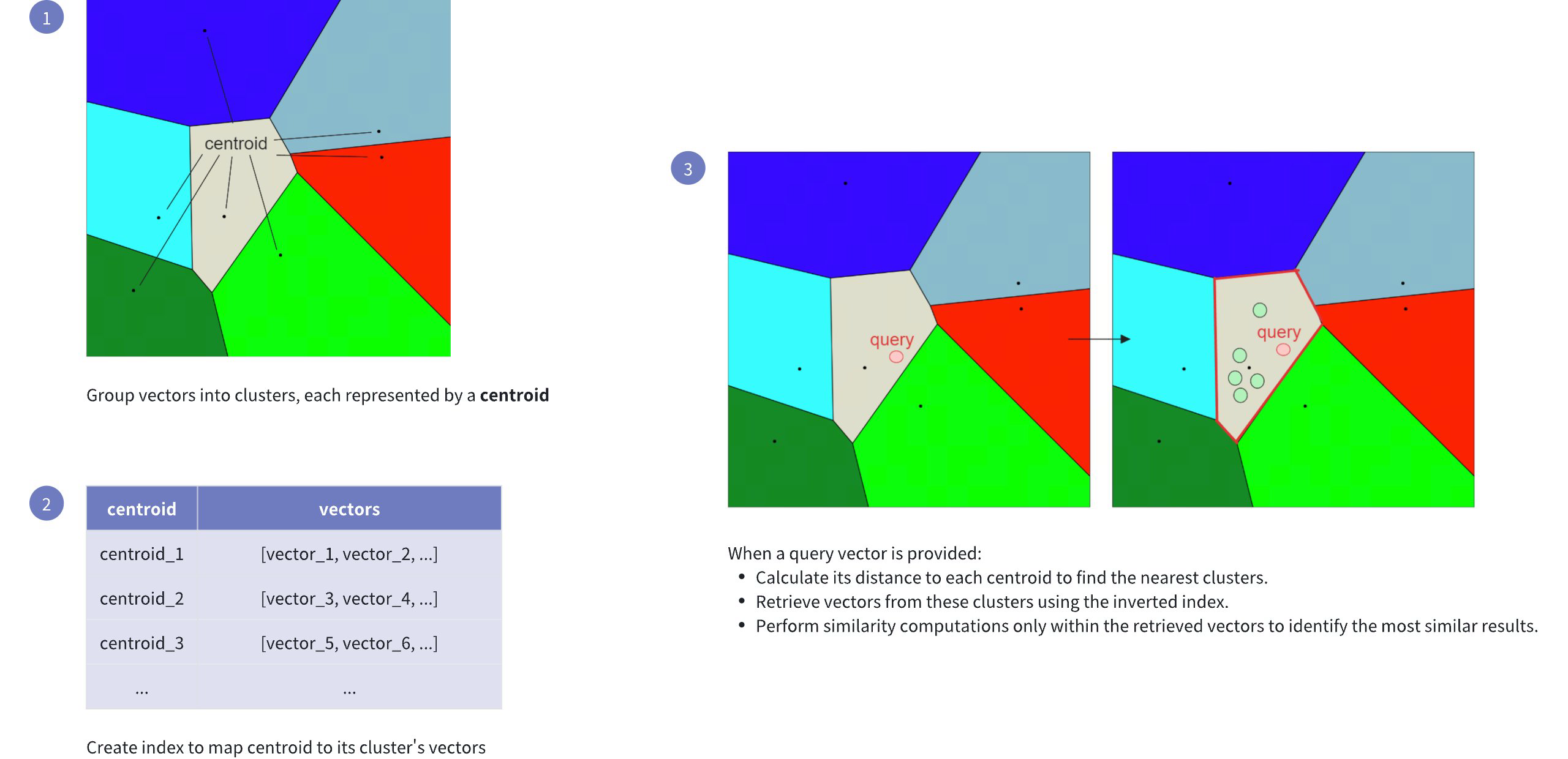
This indexing method speeds up the search process, but it comes with a potential drawback: the candidate found as the nearest to the query embedding may not be the exact nearest one. This can happen if the nearest embedding to the query embedding resides in a cluster different from the one selected based on the nearest centroid (see visualization below).
To address this issue, IVF_FLAT provides two hyperparameters that we can tune:
nlist: Specifies the number of partitions to create using the k-means algorithm.nprobe: Specifies the number of partitions to consider during the search for candidates.
Now if we set nprobe to 3 instead of 1, we get the following result:
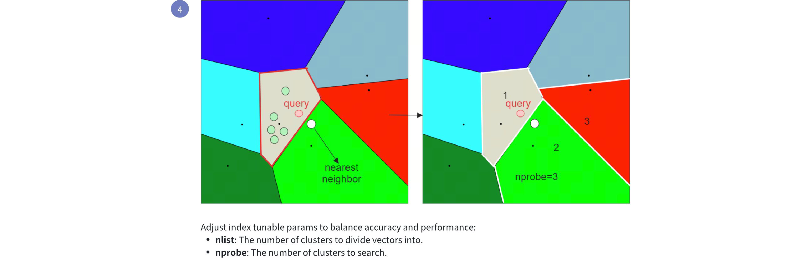
By increasing the nprobe value, you can include more partitions in the search, which can help ensure that the nearest embedding to the query is not missed, even if it resides in a different partition. However, this comes at the cost of increased search time, as more candidates need to be evaluated. For more information on index parameter tuning, refer to Index params.
# Build index
To build an IVF_FLAT index on a vector field in Milvus, use the add_index() method, specifying the index_type, metric_type, and additional parameters for the index.
from pymilvus import MilvusClient
# Prepare index building params
index_params = MilvusClient.prepare_index_params()
index_params.add_index(
field_name="your_vector_field_name", # Name of the vector field to be indexed
index_type="IVF_FLAT", # Type of the index to create
index_name="vector_index", # Name of the index to create
metric_type="L2", # Metric type used to measure similarity
params={
"nlist": 64, # Number of clusters for the index
} # Index building params
)
2
3
4
5
6
7
8
9
10
11
12
13
14
In this configuration:
index_type: The type of index to be built. In this example, set the value toIVF_FLAT.metric_type: The method used to calculate the distance between vectors. Supported values includeCOSINE,L2, andIP. For details, refer to Metric Types.params: Additional configuration options for building the index.nlist: Number of clusters to divide the dataset.
To Learn more building parameters available for the
IVF_FLATindex, refer to Index building params.
Once the index parameters are configured, you can create the index by using the create_index() method directly or passing the index params in the create_collection method. For details, refer to Create Collection.
# Search on index
Once the index is built and entities are inserted, you can perform similarity searches on the index.
search_params = {
"params": {
"nprobe": 10, # Number of clusters to search
}
}
res = MilvusClient.search(
collection_name="your_collection_name", # Collection name
anns_field="vector_field",
data=[[0.1, 0.2, 0.3, 0.4, 0.5]], # Query vector
limit=3, # TopK results to return
search_params=search_params
)
2
3
4
5
6
7
8
9
10
11
12
13
In this configuration:
params: Additional configuration options for searching on the index.nprobe: Number of clusters to search for.
To learn more search parameters available for the IVF_FLAT index, refer to Index-Specific search params.
# Index params
This section provides an overview of the parameters used for building an index and performing searches on the index.
# Index building params
The following table lists the parameters that can be configured in params when building an index.
| Parameter | Description | Value Range | Tuning Suggestion |
|---|---|---|---|
nlist | The number of clusters to create using the k-means algorithm during index building. Each cluster, represented by a centroid, stores a list of vectors. Increasing this parameter reduces the number of vectors in each cluster, creating smaller, more focused partitions. | Type: Integer Range: [1, 65536] Default Value: 128 | Larger nlist vlaues improve recall by creating more refined clusters but increase index building time. Optimize based on dataset size and available resources. In most cases, we recommend you set a value within this range: [32, 4096]. |
# Index-specific search params
The following table lists the parameters that can be configured in search_params.params when searching on the index.
| Parameter | Description | Value Range | Tuning Suggestion |
|---|---|---|---|
nprobe | The number of clusters to search for candidates. Higher values allow more clusters to be searched, improving recall by expanding the search scope but at the cost of increased query latency. | Type: Integer Range: [1, nlist] Default value: 8 | Increasing this value improves recall but may slow down the search. Set nprobe proportionally to nlist to balance speed and accuracy. In most cases, we recommend you set a value within this range: [1, nlist]. |
# IVF_SQ8
The IVF_SQ8 index is a quantization-based indexing algorithm designed to tackle large-scale similarity search challenges. This index type achieves faster searches with a much smaller memory footprint compared to exhaustive search methods.
# Overview
The IVF_SQ8 index is built on two key components:
- Inverted File (IVF): Organizes the data into clusters, enabling the search algorithm to focus only on the most relevant subsets of vectors.
- Scalar Quantization (SQ8): Compresses the vectors to a more compact form, drastically reducing memory usage while maintaining enough precision for fast similarity calculations.
# IVF
IVF is like creating an index in a book. Instead of scanning every page (or, in our case, every vector), you look up specific keywords (clusters) in the index to quickly find the relevant pages (vectors). In our scenario, vectors are grouped into clusters, and the algorithm will search within a few clusters that are close to the query vector.
Here's how it works:
- Clustering: Your vector dataset is divided into a specified number of clusters, using a clustering algorithm like k-means. Each cluster has a centroid (a representative vector for the cluster).
- Assignment: Each vector is assigned to the cluster whose centroid is closest to it.
- Inverted Index: An index is created, mapping each cluster centroid to the list of vectors assigned to that cluster.
- Search: When you search for nearest neighbors, the search algorithm compares your query vector with the cluster centroids and selects the most promising cluster(s). The search is then narrowed down to the vectors within those selected clusters.
To learn more about its technical details, refer to IVF_FLAT.
# SQ8
Scalar Quentization (SQ) is a technique used to reduce the size of high-dimensional vectors by replacing their values with smaller, more compact representations. The SQ8 variant uses 8-bit integers instead of the typical 32-bit floating point numbers to store each dimension value of a vector. This greatly reduces the amount of memory required to store the data.
Here's how SQ8 works:
- Range Identification: First, identify the minmum and maximum values within the vector. This range defines the bounds for quantization.
- Normalization: Normalize the vector values to a range between 0 and 1 using the formula:
normalized_value=max−minvalue−min
This ensures all values are mapped proporitionally within a standardized range, preparing them for compression.
- 8-Bit Compression: Multiply the normalized value by 255 (the maximum value for an 8-bit integer) and round the result to the nearest integer. This effectively compresses each value into an 8-bit representation.
Suppose you have a dimension value of 1.2, with a minimum value of -1.7 and a maximum value of 2.3. The following figure shows how SQ8 is applied to convert a float32 value to an int8 integer.
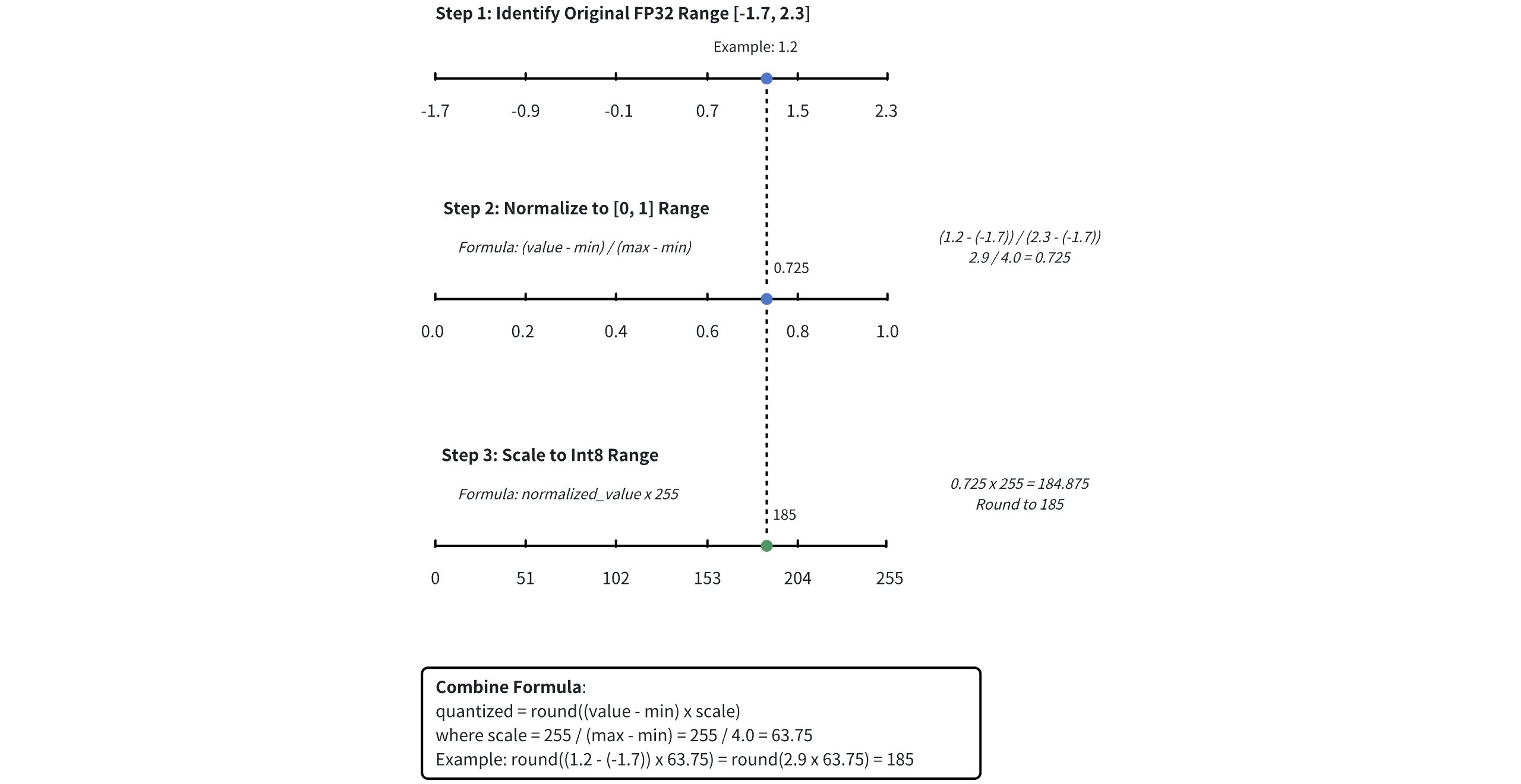
# IVF+SQ8
The IVF_SQ8 index combines IVF and SQ8 to efficiently perform similarity searches:
- IVF narrows the search scope: The dataset is divided into clusters, and when a query is issued, IVF first compares the query to the cluster centroids, selecting the most relevant clusters.
- SQ8 speeds up distance calculations: Within the selected clusters, SQ8 compreses the vectors into 8-bit integers, reducing memory usage and accelerating distance computations.
By using IVF to focus the search and SQ8 to speed up computations, IVF_SQ8 achieves both fast search times and memory efficiency.
# Build index
To build an IVF_SQ8 index on a vector field in Milvus, use the add_index() method, specifying the index_type, metric_type, and additional parameters for the index.
from pymilvus import MilvusClient
# Prepare index building params
index_params = MilvusClient.prepare_index_params()
index_params.add_index(
field_name="your_vector_field_name", # Name of the vector field to be indexed
index_type="IVF_SQ8", # Type of the index to create
index_name="vector_index", # Name of the index to create
metric_type="L2", # Metric type used to measure similarity
params={
"nlist": 64, # Number of clusters to create using the k-means algorithm during index building
} # Index building params
)
2
3
4
5
6
7
8
9
10
11
12
13
14
In this configuration:
index_type: The type of index to be built. In this example, set the value toIVF_SQ8.metric_type: The method used to calculate the distance between vectors. Supported values includeCOSINE,L2, andIP. For details, refer to Metric Types.params: Additional configuration options for building the index.nlist: Number of clusters to create using the k-means algorithm during index building.
To learn more building parameters available for the IVF_SQ8 index, refer to Index building params.
Once the index parameters are configured, you can create the index by using the create_index() method directly or passing the index params in the create_collection method. For details, refer to Create Collection.
# Search on index
Once the index is built and entities are inserted, you can perform similarity searches on the index.
search_params = {
"params": {
"nprobe": 8, # Number of clusters to search for candidates
}
}
res = MilvusClient.search(
collection_name="your_collection_name", # Collection name
anns_field="vector_field", # Vector field name
data=[[0.1, 0.2, 0.3, 0.4, 0.5]], # Query vector
limit=10, # TopK results to return
search_params=search_params
)
2
3
4
5
6
7
8
9
10
11
12
13
In this configuration:
params: Additional configuration options for searching on the index.nprobe: Number of clusters to search for candidates.
To learn more search parameters available for the IVF_SQ8 index, refer to Index-specific search params.
# Index params
This section provides an overview of the parameters used for building an index and performing searches on the index.
# Index building params
The following table lists the parameters that can be configured in params when building an index.
| Index | Parameter | Description | Value Range | Tuning Suggestion |
|---|---|---|---|---|
| IVF | nlist | The number of clusters to create using the k-means algorithm during index building. | Type: Integer Range: [1, 65536] Default value: 128 | Larger nlist values improve recall by creating more refined clusters but increase index building time. Optimize based on dataset size and available resources. In most cases, we recommend you set a value within this range: [32, 4096]. |
# Index-specific search params
The following table lists the parameters that can be configured in search_params.params when searching on the index.
| Index | Parameter | Description | Value Range | Tuning Suggestion |
|---|---|---|---|---|
| IVF | nprobe | The number of clusters to search for candidates. | Type: Integer Range: [1, nlist] Default value: 8 | Higher values allow more clusters to be searched, imporving recall by expanding the search scope but at the cost of increased query latency. Set nprobe proportionally to nlist to balance speed and accuracy. In most cases, we recommend you set a value within this range: [1, nlist]. |
# IVF_PQ
The IVF_PQ index is a quantization-based indexing algorithm for approximate nearest neighbor search in high-dimensional spaces. While not as fast as some graph-based methods, IVF_PQ often requires significantly less memory, making it a practical choice for large datasets.
# Overview
The IVF_PQ stands for Inverted File Product Quantization, a hybrid approach that combines indexing and compression for efficient vector search and retrieval. It leverages two core components: Inverted File(IVF) and Product Quantization(PQ).
# IVF
IVF is like creation an index in a book. Instead of scanning every page (or, in our case, every vector), you look up specific keywords (clusters) in the index to quickly find the relevant pages (vectors). In our scenario, vectors are grouped into clusters, and the algorithm will search within a few clusters that are close to the query vector.
Here's how it works:
- Clustering: Your vector dataset is divided into a specified number of clusters, using a clustering algorithm like k-means. Each cluster has a centroid (a representative vector for the cluster).
- Assignment: Each vector is assigned to the cluster whose centroid is closest to it.
- Inverted Index: An index is created, mapping each cluster centroid to the list of vectors assigned to that cluster.
- Search: When you search for nearest neighbors, the search algorithm compares your query vector with the cluster centroids and selects the most promising cluster(s). The search is then narrowed down to the vectors within those selected clusters.
To learn more about its technical details, refer to IVF_FLAT.
# PQ
Product Quatization (PQ) is a compression method for high-dimensional vectors that significantly reduces storage requirements while enabling fast similarity search operations.
The PQ process involves these key stages:
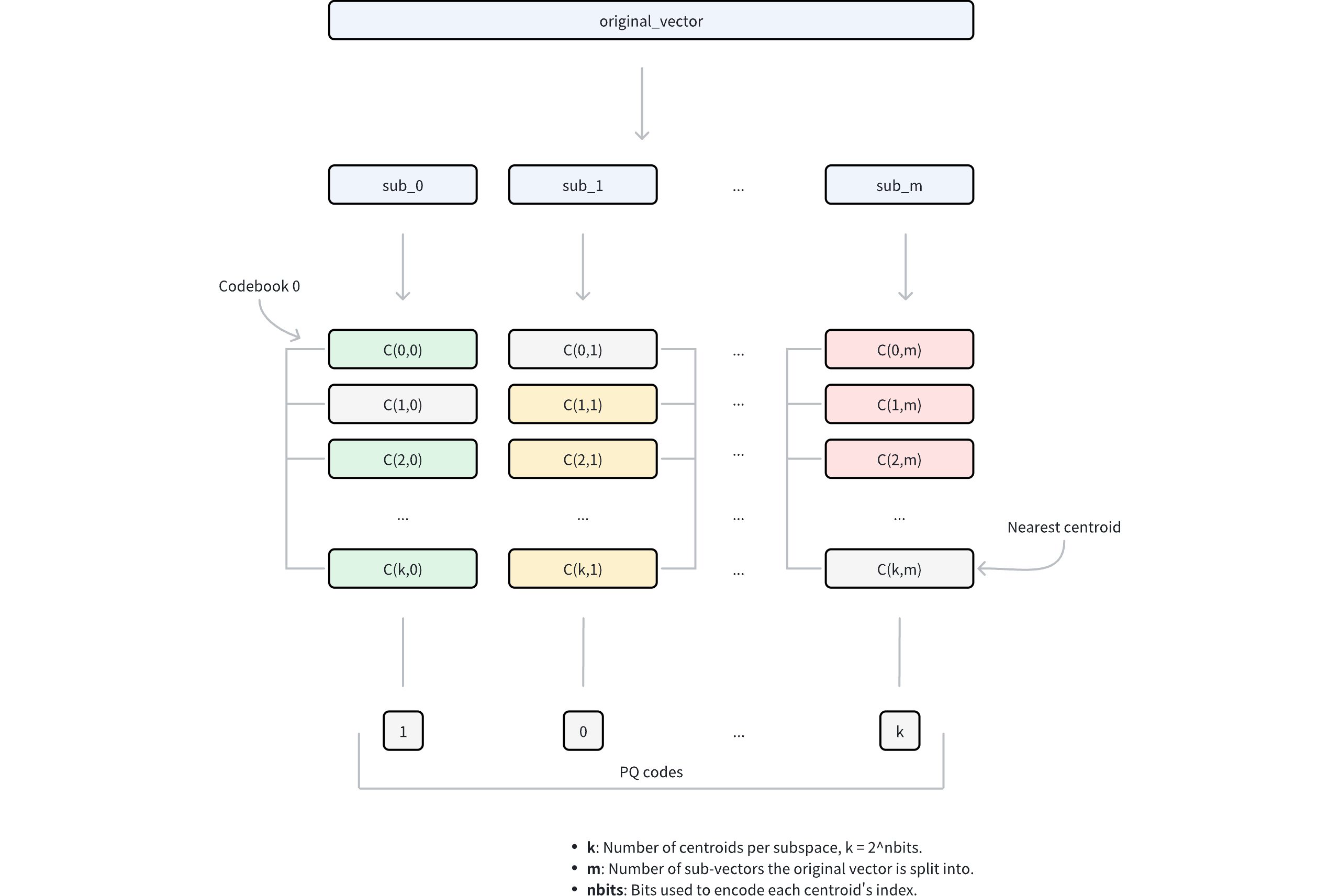
- Dimension decomposition: The algorithm begins by decomposing each high-dimensional vector into
mequal-sized sub-vectors. This decomposition transforms the original D-dimensional space intomdisjoint subspaces, where each subspace contains D/m dimensions. The parametermcontrols the granularity of the decomposition and directly influences the compression ratio. - Subspace codebook generation: Within each subspace, the algorithm applies k-means clustering to learn a set of representative vectors (centroids). These centroids collectively form a codebook for that subspace. The number of centroids in each codebook is determined by the parameter
nbits, where each codebook will 2nbits centroids. For example, ifnbits = 8, each codebook will contain 256 centroids. Each centroid is assigned a unique index withnbitsbits. - Vector quantization: For each sub-vector in the original vector, PQ identifies its nearest centroid within the corresponding subspace using a specific metric type. This process effectively maps each sub-vector to its closest representative vector in the codebook. Instead of storing the full sub-vector coordinates, only the index of the matched centroid is retained.
- Compressed representation: The final compressed representation consists of
mindices, one from each subspace, collectively referred to as PQ codes. This encoding reduces the storage requirement from D x 32 bits (assuming 32-bit floating-point numbers) to m x nbits bits, achieving substantial compression while preserving the ability to approximate vector distances.
For more details on parameter tuning and optimization, refer to Index params.
NOTE
Consider a vector with D = 128 dimensions usng 32-bit floating-point numbers. With PQ parameters m = 64 (sub-vectors) and nbits = 8 (thus k=28=256 centroids per subspace), we can compare the storage requirements:
- Original vector: 128 dimensions x 32 bits = 4096 bits
- PQ-compressed vector: 64 sub-vectors x 8 bits = 512 bits
This represents an 8x reduction in storage requirements.
Distance computation with PQ: When performing similarity search with a query vector, PQ enables efficient computation through the following steps:
Query preprocessing:
- The query vector is decomposed into
msub-vectors, matching the original PQ decomposition structure. - For each query sub-vector and its corresponding codebook (containing 2nbits centroids), compute and store distances to all centroids.
- This generates
mlookup tables, where each table contains 2nbits distances.
- The query vector is decomposed into
Distance approximation: For any database vector represented by PQ codes, its approximate distance to the query vector is computed as follows:
- For each of the
msub-vectors, retrieve the pre-computed distance from the corresponding lookup table using the stored centroid idnex. - Sum these
mdistances to obtain the approximate distance based on a specific metric type (e.g. Euclidean distance).
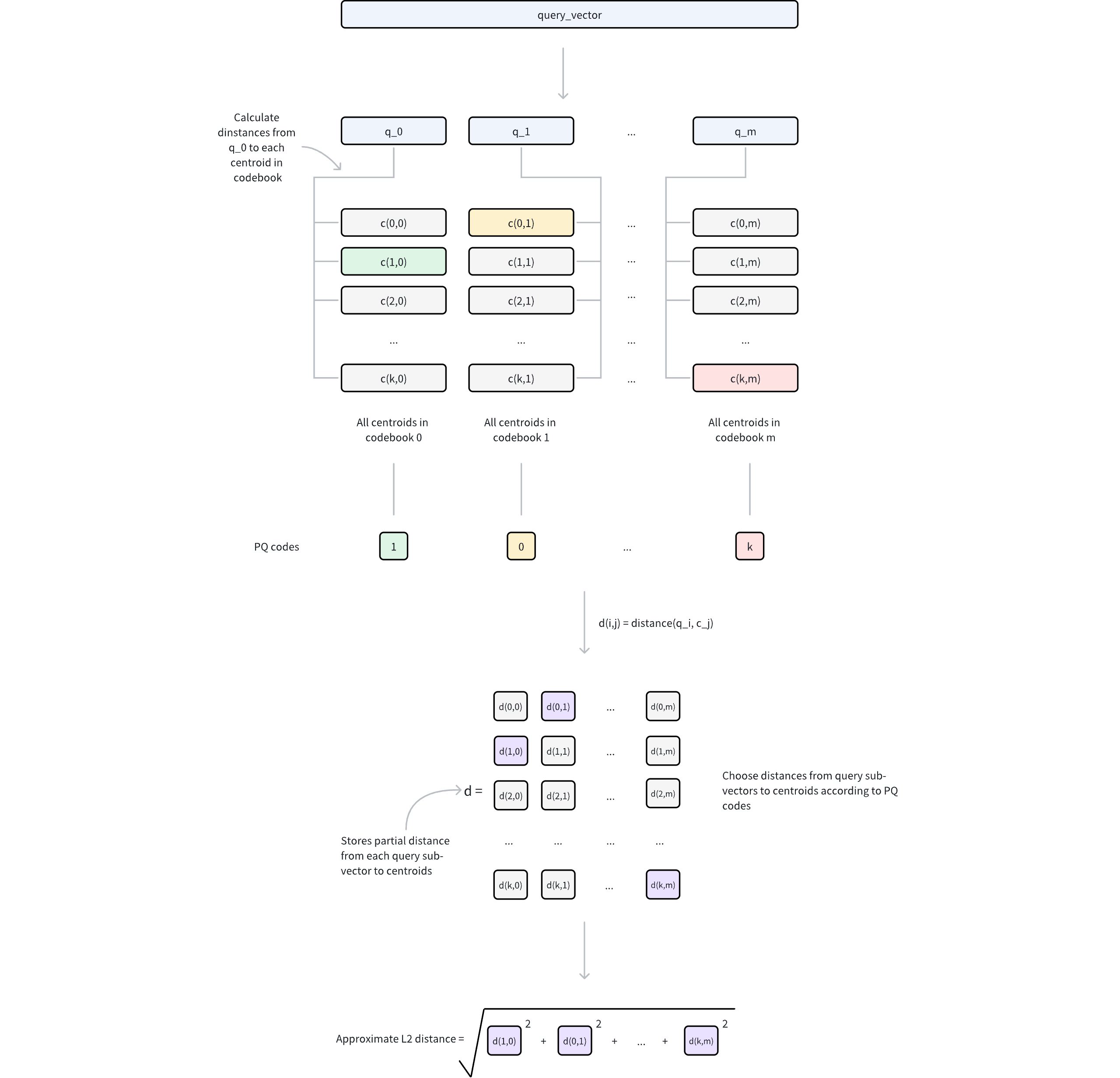
- For each of the
# IVF + PQ
The IVF_PQ index combines the strengths of IVF and PQ to accelerate searches. The process works in two steps:
- Coarse filtering with IVF: IVF partitions the vector space into clusters, reducing the search scope. Instead of evaluating the entire dataset, the algorithm focuses only on the clusters closest to the query vector.
- Fine-grained comparison with PQ: Within the selected clusters, PQ uses compressed and quantized vector representations to compute approximate distances quickly.
The performance of the IVF_PQ index is significantly impacted by the parameters that control both the IVF and PQ algorithms. Tuning these parameters is crucial to achieve the optimal results for a given dataset and application. More detailed information about these parameters and how to tune them can be found in Index params.
# Build index
To build an IVF_PQ index on a vector field in Milvus, use the add_index() method, specifying the index_type, metric_type, and additional parameters for the index.
from pymilvus import MilvusClient
index_params = MilvusClient.prepare_index_params()
index_params.add_index(
field_name="your_vector_field_name", # Name of the vector field to be indexed
index_type="IVF_PQ", # Type of the index to create
index_name="vector_index", # Name of the index to create
metric_type="L2", # Metric type used to measure similarity
params={
"m": 4, # Number of sub-vectors to split eahc vector into
} # Index building params
)
2
3
4
5
6
7
8
9
10
11
12
13
In this configuration:
index_type: The type of index to be built. In this exmaple, set the value toIVF_PQ.metric_type: The method used to calculate the distance between vectors. Supported values includeCOSINE,L2, andIP. For detail, refer to Metric Types.params: Additional configuration options for building the index.m: Number of sub-vectors to split the vector into.
To learn more building parameters available for the IVR_PQ index, refer to Index building params.
Once the index parameters are configured, you can create the index by using the create_index() method directly or passing the index params in the create_collection method. For details, refer to Create Collection.
# Search on index
Once the index is built and entities are inserted, you can perform similarity searches on the index.
search_params = {
"params": {
"nprobe": 10, # Number of clusters to search
}
}
res = MilvusClient.search(
collection_name="your_collection_name", # Collection name
anns_field="vector_field", # Vector field name
data=[[0.1, 0.2, 0.3, 0.4, 0.5]], # Query vector
limit=3, # TopK results to return
search_params=search_params
)
2
3
4
5
6
7
8
9
10
11
12
13
In this configuration:
params: Additional configuration options for searching on the index.nprobe: Number of clusters to search for.
To learn more search parameters available for the IVF_PQ index, refer to Index-specific search params.
# Index params
This section provides an overview of the parameters used for building an index and performing searches on the index.
# Index building params
The following table lists the parameters that can be configured in params when building an index.
| Index | Parameter | Description | Value Range | Tuning Suggestion |
|---|---|---|---|---|
| IVF | nlist | The number of clusters to create using the k-means algorithm during index building. | Type: Integer Range: [1, 65536] Default value: 128 | Larger nlist values improve recall by creating more refined clusters but increase index building time. Optimize based on dataset size and available resources. In most cases, we recommend you set a value within this range: [32, 4096]. |
| PQ | m | The number of sub-vectors (used for quantization) to divide each high-dimensional vector into during the quantization process. | Type: Integer Range: [1, 65536] Default value: None | A higher m value can improve accuracy, but it also increases the computational complexity and memory usage. m must be a divisor of the vector dimension (D) to ensure proper decomposition. A commonly recommended value is m = D/2. In most cases, we recommend you set a value within this range: [D/8, D]. |
| PQ | nbits | The number of bits used to represent each sub-vector's centroid index in the compressed form. It directly determines the size of each codebook. Each codebook will contain 2nbits centroids. For example, if nbits is set to 8, each sub-vector will be represented by an 8-bit centroid's index. This allows for 28 (256) possible centroids in the codebook for that sub-vector. | Type: Integer Range: [1, 64] Default value: 8 | A higher nbits value allows for larger codebooks, potentially leading to more accurate representations of the original vectors. However, it also means using more bits to store each index, resulting in less compression. In most cases, we recommend you set a value within this range: [1, 16]. |
# Index-specific search params
The following table lists the parameters that can be configured in search_params.params when searching on the index.
| Index | Parameter | Description | Value Range | Tuning Suggestion |
|---|---|---|---|---|
| IVF | nprobe | The number of clusters to search for candidates. | Type: Integer Range: [1, nlist] Default value: 8 | Higher values allow more clusters to be searched, improving recall by expanding the search scope but at the cost of increased query latency. Set nprobe proportionally to nlist to balance speed and accuracy. In most cases, we recommend you set a value within this range: [1, nlist]. |
# IVF_RABITQ
The IVF_RABITQ index is a binary quantization-based indexing algorithm that quantizes FP32 vectors into binary representations. This index offers exceptional storage efficiency with a 1-to-32 compression ratio while maintaining relatively good recall rates. It supports optional refinement to achieve higher recall at the cost of additional stroage, making it a versatile replacement for IVF_SQ8 and IVF_FLAT in memory-constrained scenarios.
# Overview
The IVF_RABITQ stands for Inverted File with RaBitQ quantization, combining two powerful techniques for efficient vector search and storage.
# IVF
Inverted File (IVF) organizes the vector space into manageable regions using k-means clustering. Each cluster is represented by a centroid, serving as a reference point for the vectors within that cluster. This clustering approach reduces the search space by allowing the algorithm to focus only on the most relevant clusters during query processing.
To learn more about LVF technical details, refer to IVF_FLAT.
# RaBitQ
RaBitQ is a state-of-the-art binary quantization method with theoretical guarantees, introduced in the research paper "RaBitQ: Quantizing High-Dimensional Vectors with a Theoretical Error Bound for Approximate Nearest Neighbor Search" by Jianyang Gao and Cheng Long.
RaBitQ introduces several innovative concepts:
Angular Information Encoding: Unlike traditional spatial encoding, RaBitQ encodes angular information through vector normalization. In IVF_RABITQ, data vectors are normalized against their nearest IVF centroid, enhancing the precision of the quantization process.
Theoretical Foundation: The core distance approximation formula is:
∥or−qr∥2≈∥or−co∥2+∥qr−co∥2−2⋅C(or,co)⋅⟨o~,qr−co⟩+C1(or,co)
Where:
- or is a data vector from the dataset
- qr is a query vector
- co is the nearest IVF centroid vector for or
- C(or,co) and C1(or,co) are precomputed constants
- o~ is the quantized binary vector stored in the index
- ⟨o~,qr−co⟩ represents the dot-product operation
Computational Efficiency: The binary nature of o~ makes distance calculations extremely fast, particularly benefiting from modern CPU architectures with dedicated AVX-512 VPOPCNTDQ instructions on Intel Ice Lake + or AMD Zen 4+ processors.
Algorithmic Enhancements: RaBitQ integrates effectively with established techniques like the FastScan approach and random rotations for improved performance.
# IVF + RaBitQ
The IVF_RABITQ index combines IVF's efficient clustering with RaBitQ's advanced binary quantization:
- Coarse Filtering: IVF partitions the vector space into clusters, significantly reducing the search scope by focusing on the most relevant cluster regions.
- Binary Quantization: Within each cluster, RaBitQ compresses vectors into binary representations
- Optional Refinement: When enabled, the index stores additional refined data using higher precision formats (SQ6, SQ8, FP16, BF16, or FP32) to improve recall rates at the cost of increased storage.
Milvus implements IVF_RABITQ using the following FAISS factory strings:
- With refinement:
"RR({dim}),IVF{nlist},RaBitQ,Refine({refine_index})" - Without refinement:
"RR({dim}),IVF{nlist},RaBitQ"
# Build index
To build an IVF_RABITQ index on a vector field in Milvus, use the add_index() method, specifying the index_type, metric_type, and additional parameters for the index.
from pymilvus import MilvusClient
# Prepare index building params
index_params = MilvusClient.prepare_index_params()
index_params.add_index(
field_name="your_vector_field_name", # Name of the vector field to be indexed
index_type="IVF_RABITQ", # Type of the index to create
index_name="vector_index", # Name of the idnex to create
metric_type="L2", # Metric type used to measure similarity
params={
"nlist": 1024, # Number of clusters for the index
"refine": True, # Enable refinement for higher recall
"refine_type": "SQ8" # Refinement data format
} # Index building params
)
2
3
4
5
6
7
8
9
10
11
12
13
14
15
16
In this configuration:
index_type: The type of index to be built. In this example, set the value toIVF_RABITQ.metric_type: The method used to calculate the distance between vectors. Supported values includeCOSINE,L2, andIP. For details, refer to Metric Types.params: Additional configuration options for building the index. For details, refer to Index building params.
Once the index parameters are configured, you can create the index by using the create_index() method directly or passing the index params in the create_collection method. For details, refer to Create Collection.
# Search on index
Once the index is built and entities are inserted, you can perform similarity searches on the index.
search_params = {
"params": {
"nprobe": 128, # Number of clusters to search
"rbq_query_bits": 0, # Query vector quantization bits
"refine_k": 1 # Refinement magnification factor
}
}
res = MilvusClient.search(
collection_name="your_collection_name", # Collection name
anns_field="vector_field", # Vector field name
data=[[0.1, 0.2, 0.3, 0.4, 0.5]], # Query vector
limit=3, # TopK results to return
search_params=search_params
)
2
3
4
5
6
7
8
9
10
11
12
13
14
15
In this configuration:
params: Additional configuration options for searching on the index. For details, refer to Index-specific search params.
NOTE
The IVF_RABITQ index heavily relies on the popcount hardware instruction for optimal performance. Modern CPU architectures such as Intel IceLake+ or AMD Zen 4+ with AVX512VPOPCNTDQ instruction sets provide significant performance inprovements for RaBitQ operations.
# Index params
This section provides an overview of the parameters used for building an index and performing searches on the index.
# Index building params
The following table lists the parameters that can be configured in params when building an index.
| Index | Parameter | Description | Value Range | Tuning Suggestion |
|---|---|---|---|---|
| IVF | nlist | The number of clusters to create using the k-means algorithm during index building. Each cluster, represented by a centroid, stores a list of vectors. Increasing this parameter reduces the number of vectors in each cluster, creating smaller, more focused partitions. | Type: Integer Range: [1, 65536] Default value: 128 | Larger nlist values improve recall by creating more refined clusters but increase index building time. Optimize based on dataset size and available resources. In most cases, we recommend you set a value within this range: [32, 4096]. |
| RaBitQ | refine | Enables the refine process and stores the refined data. | Type: Boolean Range: [true, false] Default value: false | Set to true if a 0.9+ recall rate is needed. Enabling refinement improves accuracy but increases storage requirements and index building time. |
| RaBitQ | refine_type | Defines the data representation used for refining when refine is enabled. | Type: String Range: [SQ6, SQ8, FP16, BF16, FP32] Default value: None | The listed values are presented in order of increasing recall rate, decreasing QPS, and increasing storage size. SQ8 is recommended as a starting point, offering a good balance between accuracy and resource usage. |
# Index-specific search params
The following table lists the parameters that can be configured in search_params.params when searching on the index.
| Index | Parameter | Description | Value Range | Tuning Suggestion |
|---|---|---|---|---|
| IVF | nprobe | The number of clusters to search for candidates. Higher values allow more clusters to be searched, improving recall by expanding the search scope but at the cost of increased query latency. | Type: Integer Range: [1, nlist] Default value: 8 | Increasing this value improves recall but may slow down the search. Set nprobe proportionally to nlist to balance speed and accuracy. In most cases, we recommend you set a value within this range: [1, nlist]. |
| RaBitQ | rbq_query_bits | Sets whether additional scalar quantization of a query vector is applied. If set to 0, the query is used without quantization. If set to a value within [1, 8], the query is preprocessed using n-bit scalar quantization. | Type: Integer Range: [0, 8] Default value: 0 | The default 0 value provides maximum recall rate but slowest performance. We recommend testing values 0, 8, and 6, as they provide similar recall rates with 6 being the fastest. Use smaller values for higher recall requirements. |
| RaBitQ | refine_k | The refining process uses higher quality quantization to pick the needed number of nearest neighbors from a refine_k times larger pool of candiates chosen using IVF_RABITQ | Type: Float Range: [1, float_max] Default value: 1 | Higher refine_k values decrease QPS but increase recall rate. Start with 1 and test values 2, 3, 4, and 5 to find the optimal trade-off between QPS and recall for your dataset. |
# HNSW
The HNSW index is a graph-based indexing algorithm that can improve performance when searching for high-dimensional floating vectors. It offers excellent search accuracy and low latency, while it requires high memory overhead to maintain its hierarchical graph structure.
# Overview
The Hierarchical Navigable Small World (HNSW) algorithm builds a multi-layered graph, kind of like a map with different zoom levels. The bottom layer contains all the data points, while the upper layers consists of a subset of data points sampled from the lower layer.
In this hierarchy, each layer contains nodes representing data points, connected by edges that indicate their proximity. The higher layers provide long-distance jumps to quickly get close to the target, while the lower layers enable a finegrained search for the most accurate results.
Here's how it works:
- Entry point: The search starts at a fixed entry point at the top layer, which is a pre-determined node in the graph.
- Greedy search: The algorithm greedily moves to the closest neighbor at the current layer until it cannot get any closer to the query vector. The upper layers serve a navigational purpose, acting as a coarse filter to locate potential entry point for the finer search at the lower levels.
- Layer descend: Once a local minimum is reached at the current layer, the algorithm jumps down to the lower layer, using a pre-established connection, and repeats the greedy search.
- Final refinement: This process continues until the bottom layer is reached, where a final refinement step identifies the nearest neighbors.
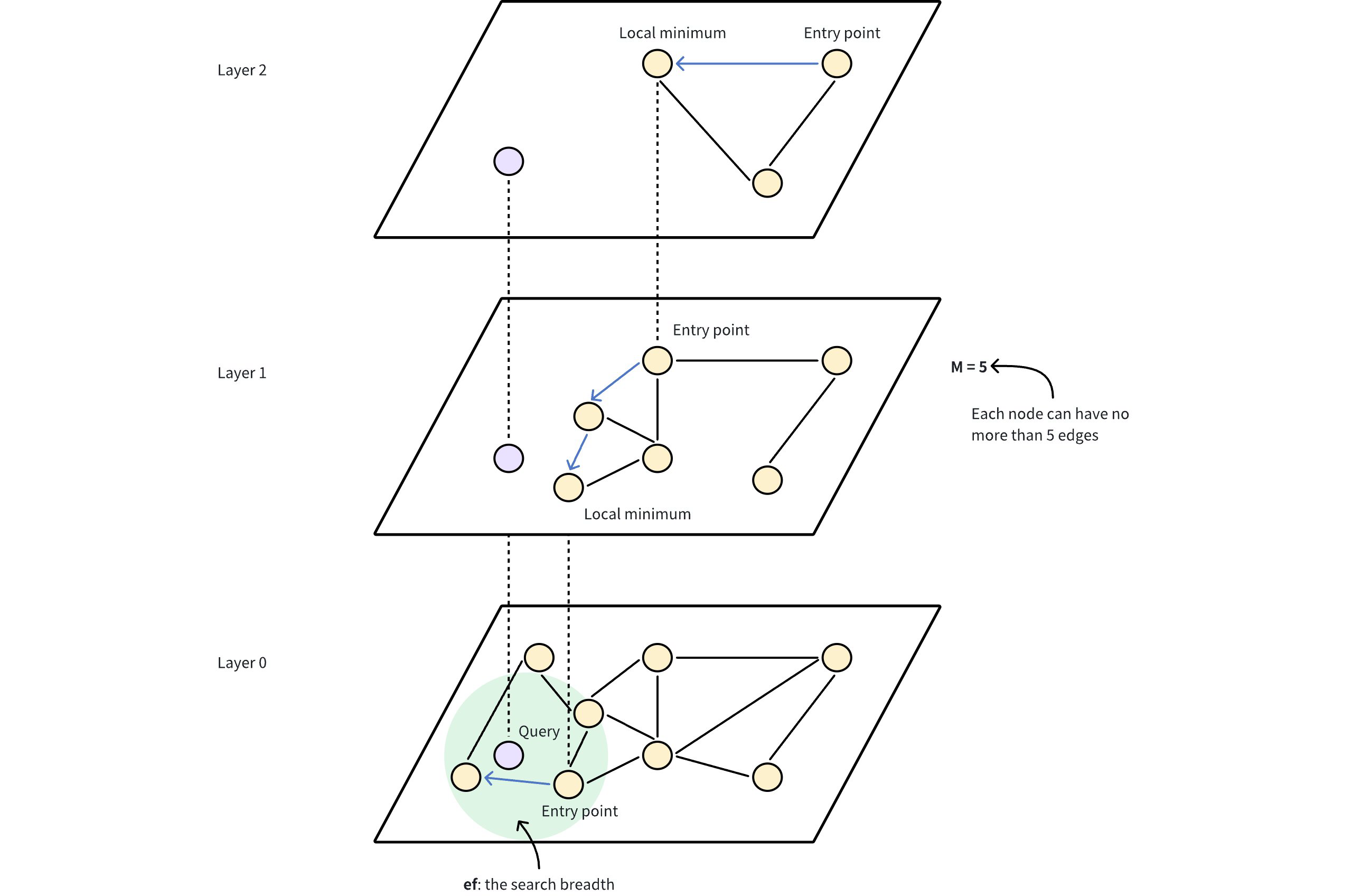
The performance of HNSW depends on several key parameters that control both the structure of the graph and the search behavior. These include:
M: The maximum number of edges or connections each node can have in the graph at each level of the hierarchy. A higherMresults in a denser graph and increases recall and accuracy as the search has more pathways to explore, which also consumes more memory and slows down insertion time due to additional connections. As shown in the image above, M = 5 indicates that each node in the HNSW graph is directly connected to a maximum of 5 other nodes. This creates a moderately dense graph structure where nodes have multiple pathways to reach other nodes.efConstruction: The number of cadidates considered during index construction. A higherefConstructiongenerally results in a better quality graph but requires more time to build.ef: The number of neighbors evaluated during a search. Increasingefimproves the likelihood of finding the nearest neighbors but slows down the search process.
For details on how to adjust these settings to suit your needs, refer to Index params.
# Build index
To build an HNSW index on a vector field in Milvus, use the add_index() method, specifying the index_type, metric_type, and additonal perameters for the index.
from pymilvus import MilvusClient
# Prepare index building params
index_params = MilvusClient.prepare_index_params()
index_params.add_index(
field_name="your_vector_field_name", # Name of the vector field to be indexed
index_type="HNSW", # Type of the index to create
index_name="vector_index", # Name of the index to create
metric_type="L2", # Metric type used to measure similarity
params={
"M": 64, # Maximum number of neighbors each node can connect to in the graph
"efConstruction": 100 # Number of candidate neighbors considered for connection during index construction
} # Index building params
)
2
3
4
5
6
7
8
9
10
11
12
13
14
15
In this configuration:
index_type: The type of index to be built. In this example, set the value toHNSW.metric_type: The method used to calculate the distance between vectors. Supported values includeCOSINE,L2, andIP. For details, refer to Metric Types.params: Additional configuration options for building the index.M: Maximum number of neighbors each node can connect to.efConstruction: Number of candidate neighbors considered for connection during index construction.
To learn more building parameters available for the HNSW index, refer to Index building params.
Once the index parameters are configured, you can create the index by using the create_index() method directly or passing the index params in the create_collection method. For details, refer to Create Collection.
# Search on index
Once the index is built and entities are inserted, you can perform similarity searches on the index.
search_params = {
"params": {
"ef": 10, # Number of neighbors to consider during the search
}
}
res = MilvusClient.search(
collection_name="your_collection_name", # Collection name
anns_field="vector_field", # Vector field name
data=[[0.1, 0.2, 0.3, 0.4, 0.5]], # Query vector
limit=10, # TopK results to return
search_params=search_params
)
2
3
4
5
6
7
8
9
10
11
12
13
In this configuration:
params: Addtional configuration options for searching on the index.ef: Number of neighbors to consider during a search.
To learn more search parameters available for the HNSW index, refer to Index-specific search params.
# Index params
This section provides an overview of the parameters used for building an index and performing searches on the index.
# Index building params
The following table lists the parameters that can be configured in params when building an index.
| Parameter | Description | Value Range | Tuning Suggestion |
|---|---|---|---|
M | Maximum number of connections (or edges) each node can have in the graph, including both outgoing and incoming edges. This parameter directly affects both index construction and search. | Type: Integer Range: [2, 2024] Default value: 30 (up to 30 outgoing and 30 incoming edges per node) | A larger M generally leads to higher accuracy but increases memory overhead and slows down both index building and search. Consider increasing M for datasets with high dimensionality or when high recall is crucial. Consider decreasing M when memory usage and search speed are primary concerns. In most cases, we recommend you set a value within this range: [5, 100]. |
efConstruction | Number of candidate neighbors considered for connection during index construction. A larger pool of candidates is evaluated for each new element, but the maximum number of connections actually established is still limited by M. | Type: Integer Range: [1, int_max] Default value: 360 | A higher efConstruction typicall results in a more accurate index, as more potential connections are explored. However, this also leads to longer indexing time and increased memory usage during construction. Consider increasing efConstruction for improved accuracy, especially in scenarios where indexing time is less critical. Consider decreasing efConstruction to speed up index construction when resource constraints are a concern. In most cases, we recommend you set a value within this range: [50, 500]. |
# Index-specific search params
The following table lists the parameters that can be configured in search_params.params when searching on the index.
| Parameter | Description | Value Range | Tuning Suggestion |
|---|---|---|---|
ef | Controls the breadth of search during nearest neighbor retrieval. It determines how many nodes are visited and evaluated as potential nearest neighbors. This parameter affects only the search process and applies exclusively to the bootom layer of the graph. | Type: Integer Range: [1, int_max] Default value: limit (TopK nearest neighbors to return) | A larger ef generally leads to higher search accuracy as more potential neighbors are considered. However, this also increases search time. Consider increasing ef when achieving high recall is critial and search speed is less of a concern. Consider decreasing ef to prioritize faster searches, especially in scenarios where a slight reduction in accuracy is acceptable. In most cases, we recommend you set a value within this range: [K, 10K]. |
# HNSW_SQ
HNSW_SQ combines Hierarchical Navigable Small World (HNSW) graphs with Scalar Quantization (SQ), creating an advanced vector indexing method that offers a controllable size-versus-accuracy trade-off. Compared to standard HNSW, this index type maintains high query processing speed while introducing a slight increase in index construction time.
# Overview
HNSW_SQ combines two indexing techniques: HNSW for fast graph-based navigation and SQ for efficient vector compression.
# HNSW
HNSW constructs a multi-layer graph where each node corresponds to a vector in the dataset. In this graph, nodes are connected based on their similarity, enabling rapid traversal through the data space. The hierarchical strcuture allows the search algorithm to arrow down the candidate neighbors, significantly accelerating the search process in high-dimensional spaces.
For more information, refer to HNSW.
# SQ
SQ is a method for compressing vectors by representing them with fewer bits. For instance:
- SQ8 uses 8 bits, mapping values into 256 levels. For more information, refer to IVF_SQ8.
- SQ6 uses 6 bits to represent each floating-point value, resulting in 64 discrete levels.
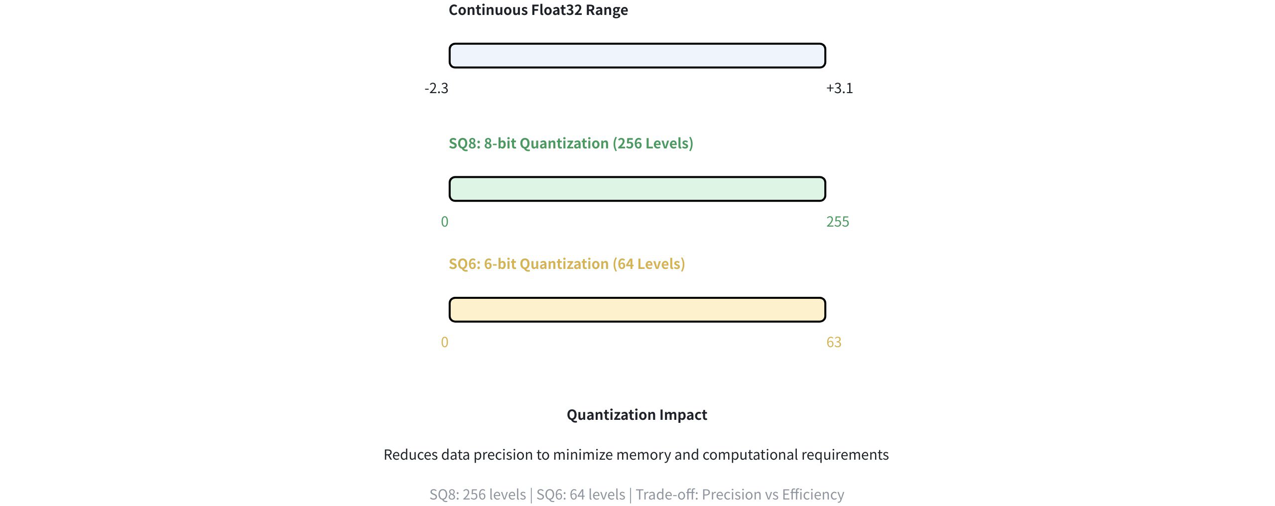
This reduction in precision dramatically decreases the memory footprint and speeds up the computation while retaining the essential structure of the data.
# HNSW + SQ
HNSW_SQ combines the strenghts of HNSW and SQ to enable efficient approximate nearest neighbor search. Here's how the process works:
- Data Compression: SQ compresses the vectors using the
sq_type(for example, SQ6 or SQ8), which reduces memory usage. This compression may lower precision, but it allows the system to handle larger datasets. - Graph Construction: The compressed vectors are used to build an HNSW graph. Because the data is compressed, the resulting graph is smaller and faster to search.
- Candidate Retrieval: When a query vector is provided, the algorithm uses the compressed data to quickly identify a pool of candidate neighbors from the HNSW graph.
- (Optional) Result Refinement: The initial candidate results can be refined for better accuracy, based on the following parameters:
refine: Controls whether this refinement step is activated. When set totrue, the system recalculates distances using higher-precision or uncompressed representations.refine_type: Specifies the precision level of data used during refinement (e.g., SQ6, SQ8, BF16). A higher-precision choice such asFP32can yield more accurate results but requires more memory. This must exceed the precision of the original compressed data set bysq_type.refine_k: Acts as a magnification factor. For instance, if your top k is 100 andrefine_kis 2, the system reranks the top 200 candidates and returns the best 100, enhancing overall accuracy.
For a full list of parameters and valid values, refer to Index params.
# Build index
To build an HNSQ_SQ index on a vector field in Milvus, use the add_index() method, specifying the index_type, metric_type, and additional parameters for the index.
from pymilvus import MilvusClient
# Prepare index building params
index_params = MilvusClient.prepare_index_params()
index_params.add_index(
field_name="your_vector_field_name", # Name of the vector field to be indexed
index_type="HNSW_SQ", # Type of the index to create
index_name="vector_index", # Name of the index to create
metric_type="L2", # Metric type used to measure similarity
params={
"M": 64, # Maximum number of neighbors each node can connect to in the graph
"efConstruction": 100, # Number of candidate neighbors considered for connection during index construction
"sq_type": "SQ6", # Scalar quantizer type
"refine": True, # Whether to enable the refinement step
"refine_type": "SQ8" # Precision level of data used for refinement
} # Index building params
)
2
3
4
5
6
7
8
9
10
11
12
13
14
15
16
17
18
In this configuration:
index_type: The type of index to be built. In this example, set the value toHNSW_SQ.metric_type: The method used to calculate the distance between vectors. Supported values includeCOSINE,L2, andIP. For details, refer to Metric Types.params: Additional configuration options for building the index. For details, refer to Index building params.
Once the index parameters are configured, you can create the index by using the create_index() method directly or passing the index params in the create_collection method. For details, refer to Create Collection.
# Search on index
Once the index is built and entities are inserted, you can perform similarity searches on the index.
search_params = {
"params": {
"ef": 10, # Parameter controlling query time/accuracy trade-off
"refine_k": 1 # The magnification factor
}
}
res = MilvusClient.search(
collection_name="your_collection_name", # Collection name
anns_field="vector_field", # Vector field name
data=[[0.1, 0.2, 0.3, 0.4, 0.5]], # Query vector
limit=3, # TopK results to return
search_params=search_params
)
2
3
4
5
6
7
8
9
10
11
12
13
14
This this configuration:
params: Additional configuration options for searching on the index. For details, refer to Index-specific search params.
# Index params
This section provides an overview of the parameters used for building an index and performing searches on the index.
# Index building params
The following table lists the parameters that can be configured in params when building an index.
| Index | Parameter | Description | Value Range | Tuning Suggestion |
|---|---|---|---|---|
| HNSW | M | Maximum number of connections (or edges) each node can have in the graph, including both outgoing and incoming edges. This parameter directly affects both index construction and search. | Type: Integer Range: [2, 2048] Default value: 30 (up to 30 outgoing and 30 incoming edges per node) | A larger M generally leads to higher accuracy but increases memory overhead and slows down both index building and search. Consider increasing M for datasets with high dimensionality or when high recall is crucial. Consider decreasing M when memory usage and search speed are primary concerns. In most cases, we recommend you set a value within this range: [5, 100]. |
| HNSW | efConstruction | Number of candidate neighbors considered for connection during index construction. A larger pool of candidates is evaluated for each new element, but the maximum number of connections actually established is still limited by M | Type: Integer Range: [1, int_max] Default value: 360 | A higher efConstruction typically results in a more accurate index, as more potential connections are explored. However, this also leads to longer indexing time and increased memory usage during construction. Consider increasing efConstruction for improved accuracy, especially in senarios where indexing time is less critical. Consider decreasing efConstruction to speed up index construction when resource constraints are a concern. In most cases, we recommend you set a value within this range: [50, 500]. |
| SQ | sq_type | Specifies the scalar quantization method for compressing vectors. Each option offers a different balance between compression and accuracy: SQ6 Encodes vectors using 6-bit integers. SQ8 Encodes vectors using 8-bit integers. BF16 Uses the Bfloat16 format. FP16 Uses the standard 16-bit floating-point format. | Type: String Range: [SQ6, SQ8, BF16, FP16] Default value: SQ8 | The choice of sq_type depends on the specific application's needs. If memory efficiency is a primary concern, SQ6 or SQ8 might be suitable. On the other hand, if accuracy is paramount, BF16 or FP16 could be preferred. |
| SQ | refine | A boolean flag that controls whether a refinement step is applied during search. Refinement involves reranking the inital results by computing exact distances between the query vector and candidates. | Type: Boolean Range: [True, False] Default value: True | Set to True if high accuracy is essential and you can tolerate slightly slower search tiems. Use False if speed is a priority and a minor compromise in accuracy is acceptable. |
| SQ | refine_type | Determines the precision of the data used for refinement. THis precision must be higher than that of the compressed vectors (as set by sq_type), affecting both the accuracy of the reranked vectors and their memory footprint. | Type: String Range: [SQ6, SQ8, BF16, FP16, FP32] Default value: None | Use FP32 for maximum precision at a higher memory cost, or SQ6/SQ8 for better compression. BF16 and FP16 offer a balanced alternative. |
# Index-specific search params
The following table lists the parameters that can be configured in search_params.params when searching on the index.
| Index | Parameter | Description | Value Range | Tuning Suggestion |
|---|---|---|---|---|
| HNSW | ef | Controls the breadth of search during nearest neighbor retrieval. It determines how many nodes are visited and evaluated as potential nearest neighbors. This parameter affects only the search process and applies exclusively to the bottom layer of the graph. | Type: Integer Range: [1, int_max] Default value: limit (TopK nearest neighbors to return) | A larger ef generally leads to higher search accuracy as more potential neighbors are considered. However, this also increases search time. Consider increasing ef when achieving high recall is critical and search speed is less of a concern. Consider decreasing ef to prioritize faster searches, especially in scenarios where a slight reduction in accuracy is acceptable. In most cases, we recommend you set a value within this range: [K, 10K]. |
| HNSW | refine_k | The magnification factor that controls how many extra candidates are exmined during the refinement stage, relative to the requested top K results. | Type: Float Range: [1, float_max] Default value: 1 | Higher values of refine_k can improve recall and accuracy but will also increase search time and resource usage. A vlaue of 1 means the refinement process considers only the initial top K results. |
# HNSW_PQ
HNSW_PQ leverages Hierarchical Navigable Small World (HNSW) graphs with Product Quantization (PQ), creating an advanced vector indexing method that offers a controllable size-versus-accuracy trade-off. Compared to HNSW_SQ, this index type delivers a higher recall rate at the same compression level, albeit with lower query processing speed and longer index construction time.
# Overview
HNSW_PQ combines two indexing techniques: HNSW for fast graph-based navigation and PQ for efficient vector compression.
# HNSW
HNSW constructs a multi-layer graph where each node coressponds to a vector in the dataset. In this graph, nodes are connected based on their similarity, enabling rapid traversal through the data space. The hierarchical structure allows the search algorithm to narrow down the candidate neighbors, significantly accelerating the search process in high dimensional spaces.
For more information, refer to HNSW.
# PQ
PQ is a vector compression technique that breaks down high-dimensional vectors into smaller sub-vectors, which are then quantized and compressed. The compression dramatically reduces memory requirements and accelerates distance computations.
For more information, refer to IVF_PQ.
# HNSW + PQ
HNSW_PQ combines the strengths of HNSW and PQ to enable efficient approximate nearest neighbor search. It uses PQ to compress the data (thus reducing memory usage), and then builds an HNSW graph on these compressed vectors to enable rapid candidate retrieval. During the search, the algorithm can optionally refine the candidate results using higher-precision data for improved accuracy. Here's how the process works:
- Data Compression: PQ splits each vector into multiple sub-vectors and quantizes them using a codebook of centroids, controlled by parameters like
m(sub-vector count) andnbits(bits per sub-vector). - Graph Construction: The compressed vectors are then used to build an HNSW graph. Because the vectors are stored in a compressed form, the resulting graph is typically smaller, requires less memory, and can be traversed more quickly-significantly acclerating the candidate retrieval step.
- Candidate Retrieval: When a query is executed, the algorithm uses the compressed data in the HNSW graph to efficiently identify a pool of candidate neighbors. This graph-based lookup drastically reduces the number of vectors that must be considered, improving query latency compared to brute-force searches.
- (Optional) Result Refinement: The initial candidate results can be refined for better accuracy, based on the following parameters:
refine: Controls whether this refinement step is activated. When set toTrue, the system recalculates distances using higher-precision or uncompressed representations.refine_type: Specifies the precision level of data used during refinement (e.g., SQ6, SQ8, BF16). A higher-precision choice such asFP32can yield more accurate results but requires more memory. This must exceed the precision of the original compressed data set bysq_type.refine_k: Acts as a magnification factor. For instance, if your top k is 100 andrefine_kis 2, the system reranks the top 200 candidates and returns the best 100, enhancing overall accuracy.
For a full list of parameters and valid values, refer to Index params.
# Build index
To build an HNSW_PQ index on a vector field in Milvus, use the add_index() method, specifying the index_type, metric_type, and additional parameters for the index.
from pymilvus import MilvusClient
# Prepare index building params
index_params = MilvusClient.prepare_index_params()
index_params.add_index(
field_name="your_vector_field_name", # Name of the vector field to be indexed.
index_type="HNSW_PQ", # Type of the index to create
index_name="vector_name", # Name of the index to create
metric_type="L2", # Metric type used to measure similarity
params={
"M": 30, # Maximum number of neighbors each node can connect to in the graph
"efConstruction": 360, # Number of candidate neighbors considered for connection during index construction
"m": 384,
"nbits": 8,
"refine": True, # Whether to enable the refinement step
"refine_type": "SQ8" # Precision level of data used for refinement
} # Index building params
)
2
3
4
5
6
7
8
9
10
11
12
13
14
15
16
17
18
19
In this configuration:
index_type: The type of index to be built. In this example, set the value toHNSW_PQ.metric_type: The method used to calculate the distance between vectors. Supported values includeCOSINE,L2, andIP. For details, refer to Metric Types.params: Additional configuration options for building the index. For details, refer to Index building params.
Once the index parameters are configured, you can create the index by using the create_index() method directly or passing the index params in the create_collection method. For details, refer to Create Collection.
# Search on index
Once the index is built and entities are inserted, you can perform similarity searches on the index.
search_params = {
"params": {
"ef": 10, # Parameter controlling query time/accuracy trade-off
"refine_k": 1 # The magnification factor
}
}
res = MilvusClient.search(
collection_name="your_collection_name", # Collection name
anns_field="vector_field", # Vector field name
data=[[0.1, 0.2, 0.3, 0.4, 0.5]], # Query vector
limit=3, # TopK results to return
search_params=search_params
)
2
3
4
5
6
7
8
9
10
11
12
13
14
In this configuration:
params: Additional configuration options for searching on the index. For details, refer to Index-specific search params.
# Index params
This section provides an overview of the parameters used for building an index and performing searches on the index.
# Index building params
The following table lists the parameters that can be configured in params when Building an index.
| Index | Parameter | Description | Value Range | Tuning Suggestion |
|---|---|---|---|---|
| HNSW | M | Maximum number of connections (or edges) each node can have in the graph, including both outgoing and incoming edges. This parameter directly affects both index construction and search. | Type: Integer Range: [2, 2048] Default value: 30 (up to 30 outgoing and 30 incoming edges per node) | A larger M generally leads to higher accuracy but increases memory overhead and slows down both index building and search. Consider increasing M for datasets with high dimensionality or when high recall is crucial. Consider decreasing M when memory usage and search speed are primary concerns. In most cases, we recommend you set a value within this range: [5, 100]. |
| HNSW | efConstruction | Number of candidate neighbors considered for connection during index construction. A larger pool of candidates is evaluated for each new element, but the maximum number of connections actually established is still limited by M. | Type: Integer Range: [1, int_max] Default value: 360 | A higher efConstruction typically results in a more accurate index, as more potential connections are explored. However, this also leads to longer indexing time and increased memory usage during construction. Consider increasing efConstruction for improved accuracy, especially in scenarios where indexing time is less critial. Consider decreasing efConstruction to speed up index construction when resource constraints are a concern. In most cases, we recommend you set a value within this range: [50, 500]. |
| PQ | m | The number of sub-vectors (used for quantization) to divide each high-dimensional vector into during the quantization process. | Type: Integer Range: [1, 65536] Default value: None | A higher m value cna improve accuracy, but it also increases the computational complexity and memory usage. m must be a divisor of the vector dimension (D) to ensure proper decomposition. A commonly recommended value is m = D/2. In most cases, we recommend you set a value within this range: [D/8, D]. |
| PQ | nbits | The number of bits used to represent each sub-vector's centroid index in the compressed form. It directly determines the size of each codebook. Each codebook will contain 2nbits centroids. For example, if nbits is set to 8, each sub-vector will be represented by an 8-bit centroid's index. This allows for 28 (256) possible centroids in the codebook for that sub-vector. | Type: Integer Range: [1, 64] Default value: 8 | A higher nbits value allows for larger codebooks, potentially leading to more accurate representations of the original vectors. However, it also means using more bits to store each index, resulting in less compression. In most cases, we recommend you set a value within this range: [1, 16]. |
| PQ | refine | A boolean flag that controls whether a refinement step is applied during search. Refinement involves reranking the initial results by computing exact distances between query vector and candidates. | Type: Boolean Range: [True, False] Default value: False | Set to True if high accuracy is essential and you can tolerate slightly slower search times. Use False if speed is a priority and a minor compromise in accuracy is acceptable. |
| PQ | refine_type | Determines the precision of the data used during the refinement process. This precision must be higher than that of the compressed vectors (as set by m and nbits parameters). | Type: String Range: [SQ6, SQ8, BF16, FP16, FP32] Default value: None | Use FP32 for maximum precision at a higher memory cost, or SQ6/SQ8 for better compression. BF16 and FP16 offer a balanced alternative. |
# Index-specific search params
The following table lists the parameters that can be configured in search_params.params when searching on the index.
| Index | Parameter | Description | Value Range | Tuning Suggestion |
|---|---|---|---|---|
| HNSW | ef | Controls the breadth of search during nearest neighbor retrieval. It determines how many nodes are visited and evaluated as potential nearest neighbors. This parameter affects only the search process and applies exclusively to the bottom layer of the graph. | Type: Integer Range: [1, int_max] Default value: limit (TopK nearest neighbors to return) | A larger ef generally leads to higher search accuracy as more potential neighbors are considered. However, this also increases search time. Consider increasing ef when achieving high recall is critical and search speed is less of a concern. Consider decreasing ef to prioritize faster searches, especially in scenarios where a slight reduction in accuracy is acceptable. In most cases, we recommend you set a value within this range: [K, 10K]. |
| PQ | refine_k | The magnification factor that controls how many extra candidates are examined during the refinement (reranking) state, relative to the requested top K results. | Type: Float Range: [1, float_max] Default value: 1 | Higher values of refine_k can improve recall and accuracy but will also increase search time and resource usage. A value of 1 means the refinement process considers only the initial top K results. |
# HNSW_PRQ
HNSW_PRQ leverages Hierarchical Navigable Small World (HNSW) graphs with Product Residual Quantization (PRQ), offering an advanced vector indexing method that allows you to finely tune the trade-off between index size and accuracy. PRQ goes beyond traditional Product Quantization (PQ) by introducing a residual quantization (RQ) step to capture additional information, resulting in higher accuracy or more compact indexes compared to purely PQ-based methods. However, the extra steps can lead to higher computational overhead during index building and searching.
# Overview
HNSW_PRQ combines two indexing techniques: HNSW for fast graph-based navigation and PRQ for efficient vector compression.
# HNSW
HNSW constructs a multi-layer graph where each node corresponds to a vector in the dataset. In this graph, nodes are connected based on their similarity, enabling rapid traversal through the data space. The hierarchical structure allows the search algorithm to narrow down the candidate neighbors, significantly accelerating the search process in high dimensional spaces.
For more information, refer to HNSW.
# PRQ
PRQ is a multi-stage vector compression approach that combines two complementary techniques: PQ and RQ. By first splitting a high-dimensional vector into smaller sub-vectors (via PQ) and then quantizing any remaining difference (via RQ), PRQ achieves a compact yet accurate representation of the orginal data.
The following figure shows how it works.
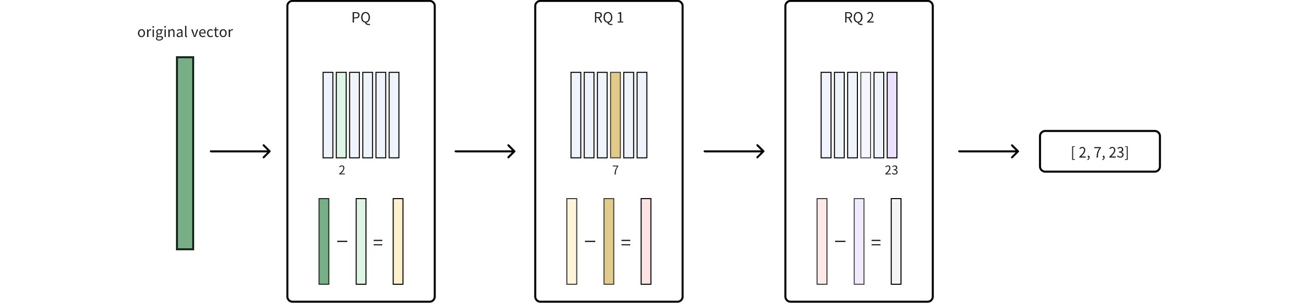
- Product Quantization (PQ): In this phase, the original vector is divided into smaller sub-vectors, and each sub-vector is mapped to its nearest centroid in a learned codebook. This mapping significantly reduces data size but introduces some rounding error since each sub-vector is approximated by a single centroid. For more details, refer to IVF_PQ.
- Residual Quantization (PQ): After the PQ stage, RQ quantizes the residual -- the difference between the original vector and its PQ-based approximation -- using additional codebooks. Because this residual is typically much smaller, it can be encoded more precisely without a large increase in storage. The parameter
nrqdetermines how many times this residual is iteratively quantized, allowing you to fine-tune the balance between compression efficiency and accuracy. - Final Compression Representation: Once RQ finishes quantizing the residual, the integer codes from both PQ and RQ are combined into a single compressed index. By capturing refined details that PQ alone might miss, RQ enhances accuracy without causing a significant increase in storage. This synergy between PQ and RQ is what defines PRQ.
# HNSW + PRQ
By combining HNSW with PRQ, HNSW_PRQ retains HNSW's fast graph-based search while taking advantage of PRQ's multi-stage compression. The workflow looks like this:
- Data Compression: Each vector is first transformed via PQ to a coarse representation, and then residuals are quantized through PQ for further refinement. The result is a set of compact codes representing each vector.
- Graph Construction: The compressed vectors (including both the PQ and RQ codes) from the basis for building the HNSW graph. Because data is stored in a compact form, the graph requires less memory, and navigation through it is accelerated.
- Candidate Retrieval: During search, HNSW uses the compressed representations to traverse the graph and retrieve a pool of candidates. This dramatically custs down the number of vectors needing consideration.
- (Optional) Result Refinement: The initial candidate results can be refined for better accuracy, based on the following parameters:
refine: Controls whether this refinement step is activated. When set totrue, the system recalculates distances using higher-precision or uncompressed representations.refine_type: Specifies the precision level of data used during refinement (e.g., SQ6, SQ8, BF16). A higher-precision choice such asFP32can yield mor eaccurate results but requires more memory. This must exceed the precision of the original compressed data set bysq_type.refine_k: Acts as a magnification factor. For instance, if your top k is 100 andrefine_kis 2, the system reranks the top 200 candidates and returns the best 100, enhancing overall accuracy.
For a full list of parameters and valid values, refer to Index params.
# Build index
To build an HNSQ_PRQ index on a vector field in Milvus, use the add_index() method, specifying the index_type, metric_type, and additional parameters for the index.
from pymilvus import MilvusClient
# Prepare index building params
index_params = MilvusClient.prepare_index_params()
index_params.add_index(
field_name="your_vector_field_name", # Name of the vector field to be indexed
index_type="HNSW_PRQ", # Type of the index to create
index_name="vector_index", # Name of the index to create
metric_type="L2", # Metric type used to measure similarity
params={
"M": 30, # Maximum number of neighbors each node can connect to in the graph
"efConstruction": 360, # Number of candidate neighbors considered for connection during index construction
"m": 384,
"nbits": 8,
"nrq": 1,
"refine": true, # Whether to enable the refinement step
"refine_type": "SQ8" # Precision level of data used for refinement
} # Index building params
)
2
3
4
5
6
7
8
9
10
11
12
13
14
15
16
17
18
19
20
In this configuration:
index_type: The type of index to be built. In this example, set the value toHNSW_PQ.metric_type: The method used to calculate the distance between vectors. Supported values includeCOSINE,L2, andIP. For details, refer to Metric Types.params: Additional configuration options for building the index. For details, refer to Index building parmas.
Once the index parameters are configured, you can create the index by using the create_index() method directly or passing the index params in the create_collection method. For details, refer to Create Collection.
# Search on index
Once the index is built and entities are inserted, you can perform similarity searches on the index.
search_params = {
"params": {
"ef": 10, # Parameter controlling query time/accuracy trade-off
"refine_k": 1 # The magnification factor
}
}
res = MilvusClient.search(
collection_name="your_collection_name", # Collection name
anns_field="vector_field", # Vector field name
data=[[0.1, 0.2, 0.3, 0.4, 0.5]], # Query vector
limit=3, # TopK results to return
search_params=search_params
)
2
3
4
5
6
7
8
9
10
11
12
13
14
In this configuration:
params: Additional configuration options for searching on the index. For details, refer to Index-specific search params
# Index params
This section provides an overview of the parameters used for building an index and perpforming searches on the index.
# Index building params
The following table lists the parameters that can be configured in params when building an index.
| Index | Parameter | Description | Value Range | Tuning Suggestion |
|---|---|---|---|---|
| HNSW | M | Maximum number of connections (or edges) each node can have in the graph, including both outgoing and incoming edges. This parameter directly affects both index construction and search. | Type: Integer Range: [2, 2048] Default value: 30 (up to 30 outgoing and 30 incoming edges per node) | A larger M generally leads to higher accuracy but increases memory overhead and slows down both index building and search. Consider increasing M for datasets with high dimensionality or when high recall is crucial. Consider decreasing M when memory usage and search speed are primary concerns. In most cases, we recommend you set a value within this range: [5, 100]. |
| HNSW | efConstruction | Number of candidate neighbors considered for connection during index construction. A larger pool of candidates is evaluated for each new element, but the maximum number of connections actually established is still limited by M. | Type: Integer Range: [1, int_max] Default value: 360 | A higher efConstruction typically results in a more accurate index, as more potential connections are explored. However, this also leads to longer indexing time and increased memory usage during construction. Consider increasing efConstruction for improved accuracy, especially in scenarios where indexing time is less critical. Consider decreasing efConstruction to speed up index construction when resource constraints are a concern. In most cases, we recommend you set a value within this range: [50, 500]. |
| PRQ | m | The number of sub-vectors (used for quantization) to divide each high-dimensional vector into during the quantization process. | Type: Integer Range: [1, 65536] Default value: None | A higher m value can improve accuracy, but it also increases the computational complexity and memory usage. m must be a divisor of the vector dimension (D) to ensure proper decomposition. A commonly recommended value is m = D/2. In most cases, we recommend you set a value within this range: [D/8, D]. |
| PRQ | nbits | The number of bits used to represent each sub-vector's centroid index in the compressed form. It directly determines the size of each codebook. Each codebook will contain 2nbits centroids. For example, if nbits is set to 8, each sub-vector will be represented by an 8-bit centroid's index. This allows for 28 (256) possible centroids in the codebook for that sub-vector. | Type: Integer Range: [1, 64] Default value: 8 | A higher nbits value allows for larger codebooks, potentially leading to more accurate representations of the original vectors. However, it also means using more bits to store each index, resulting in less compression. In most cases, we recommend you set a value within this range: [1, 16]. |
| PRQ | nrq | Controls how many residual subquantizers are used in the RQ stage. More subquantizers potentially achieve greater compression but might introduce more information loss. | Type: Integer Range: [1, 16] Default value: 2 | A higher nrq value allows for additional residual subquantization steps, potentially leading to a more precise reconstruction of the original vectors. However, it aslo means storing and computing more subquantizers, resulting in a larger index size and greater computational overhead. |
| PRQ | refine | A boolean flag that controls whether a refinement step is applied during search. Refinement involves reranking the initial results by computing exact distances between the query vector and candidates. | Type: Boolean Range: [True, False] Default value: False | Set to True if high accuracy is essential and you can tolerate slightly slower search times. Use False if speed is a priority and a minor compromise in accuracy is acceptable. |
| PRQ | refine_type | Determines the precision of the data used during the refinement process. This precision must be higher than that of the compressed vectors (as set by m and nbits parameters). | Type: String Range: [SQ6, SQ8, BF16, FP16, FP32] Default value: None | Use FP32 for maximum precision at a higher memory cost, or SQ6/SQ8 for better compression. BF16 and FP16 offer a balanced alternative. |
# Index-specific search params
The following table lists the parameters that can be configured in search_params.param when searching on the index.
| Index | Parameter | Description | Value Range | Tuning Suggestion |
|---|---|---|---|---|
| HNSW | ef | Controls the breadth of search during nearest neighbor retrieval. It determines how many nodes are visited and evaluated as potential nearest neighbors. This parameter affects only the search process and applies exclusively to the bottom layer of the graph. | Type: Integer Range: [1, int_max] Default value: limit (TopK nearest neighbors to return) | A larger ef generally leads to higher search accuracy as more potential neighbors are considered. However, this also increases search time. Consider increasing ef when achieving high recall is critial and search speed is less of a concern. Consider decreasing ef to prioritize faster searches, especially in scenarios where a slight reduction in accuracy is acceptable. In most cases, we recommend you set a value within this range: [K, 10K]. |
| PRQ | refine_k | The magnification factor that controls how many extra candidates are examined during the refinement (reranking) stage, relative to the requested top K results. | Type: Float Range: [1, float_max] Default value: 1 | Higher values of refine_k can improve recall and accuracy but will also increase search time and resource usage. A value of 1 means the refinement process considers only the initial top K results. |
# DISKANN
In large-scale scenarios, where datasets can include billions or even trillions of vectors, standard in-memory indexing methods (e.g., HNSW, IVF_FLAT) often fail to keep space due to memory limitations. DISKANN offers a disk-based approach that addresses these challenges by maintaining high search accuracy and speed when the dataset size exceeds available RAM.
# Overview
DISKANN combines two key techniques for efficient vector search:
- Vamana Graph -- A disk-based, graph-based index that connects data points (or vectors) for efficient navigation during search.
- Product Quantization (PQ) -- An in-memory compression method that reduces the size of vectors, enabling quick approximate distance calculations between vectors.
# Index construction
Vamana graph: The Vamana graph is central to DISKANN's disk-based strategy. It can handle very large datasets because it does not need to fully reside in memory during or after construction.
The following figure shows how a Vamana graph is constructed.
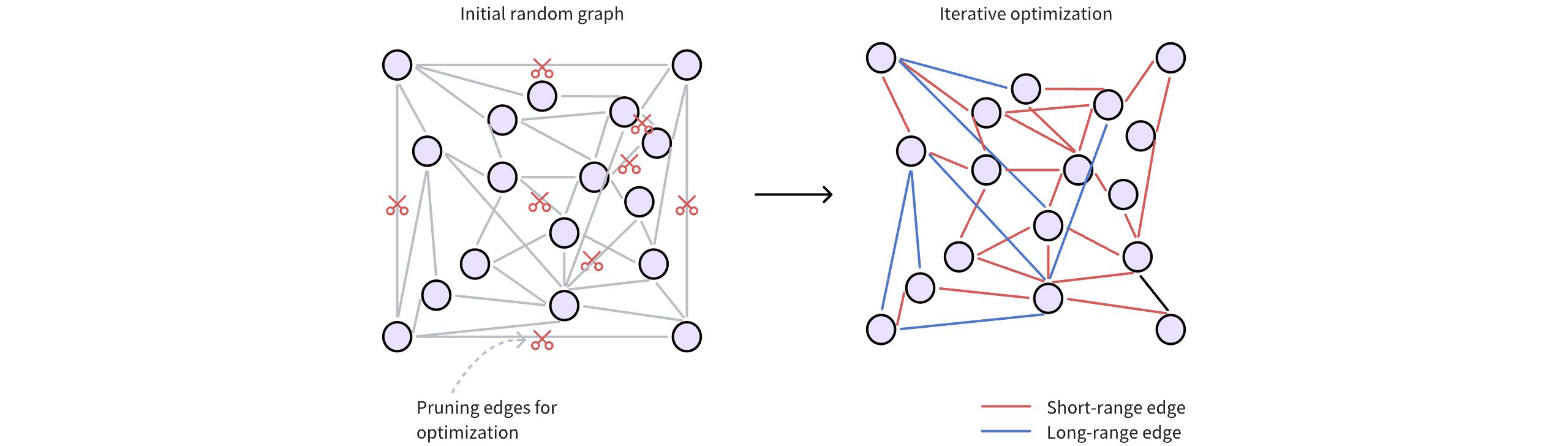
- Initial random connections: Each data point (vector) is represented as a node in the graph. These nodes are initially connected randomly, forming a dense network. Typically, a node starts with around 500 edges (or connections) for borad connectivity.
- Refining for efficiency: The initial random graph undergoes an optimization process to make it more efficient for searching. This involves two key steps:
- Pruning redundant edges: The algorithm discards unnecessary connections based on distances between nodes. This step prioritizes higher-quality edges. The
max_degreeparameter restricts the maximum number of edges per node. A highermax_degreeresults in a denser graph, potentially finding more relevant neighbors (higher recall) but also increasing memory usage and search time. - Adding strategic shortcuts: Vamana introduces long-range edges, connecting data points that are far apart in the vector space. These shortcuts allow searches to quickly jump across the graph, by passing intermediate nodes and significantly speeding up navigation. The
search_list_sizeparameter determines the breadth of the graph refinement process. A highersearch_list_sizeextends the search for neighbors during construction and can improve final accuracy, but increases index-building time.
- Pruning redundant edges: The algorithm discards unnecessary connections based on distances between nodes. This step prioritizes higher-quality edges. The
To learn more about parameter tuning, refer to DISKANN params.
PQ: DISKANN uses PQ high-dimensional vectors into smaller representations (PQ codes), which are stored in memory for rapid approximate distance calculations.
The pq_code_budget_gb_ratio parameter manages the memory footprint dedicated to storing these PQ codes. It represents a ratio between the total size of the vectors (in gigabytes) and the space allocated for storing the PQ codes. You can calculate the actual PQ code budget (in gigabytes) with this formula:
PQ Code Budget (GB) = vec_field_size_gb * pq_code_budget_gb_ratio
where:
vec_field_size_gb: is the total size of the vectors (in gigabytes).pq_code_budget_gb_ratio: is a user-defined ratio, representing the fraction of the total data size reserved for PQ codes. This parameter allows for a trade-off between search accuracy and memory resources. For more information on parameter tuning, refer to DISKANN configs.
For technical details on the underlying PQ method, refer to IVF_PQ.
# Search process
Once the index (the Vamana graph on disk and PQ codes in memory) is built, DISKANN performs ANN searches as follows:
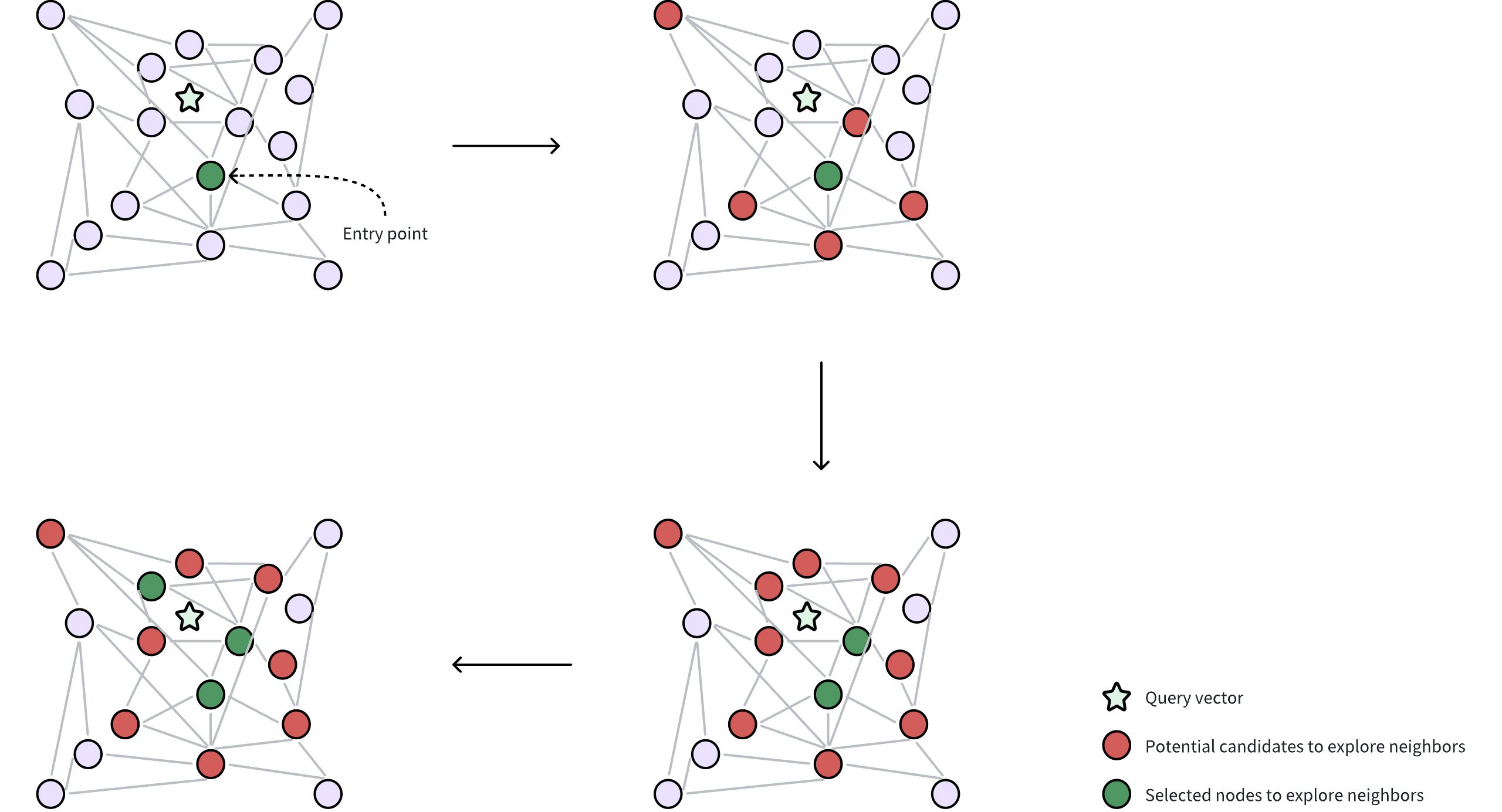
- Query and entry point: A query vector is provided to locate its nearest neighbors. DISKANN starts from a selected entry point in the Vamana graph, often a node near the global centroid of the dataset. The global centroid represents the average of all vectors, which helps to minimize the traversal distance through the graph to find desired neighbors.
- Neighborhood exploration: The algorithm gathers potential candidate neighbors (cicles in red in the figure) from the edges of the current node, leveraging in-memory PQ codes to approximate the distance between these candidates and the query vector. These potential candidate neighbors are the nodes directly connected to the selected entry point through edges in the Vamana graph.
- Selecting nodes for accurate distance calculation: From the approximate results, a subset of the most promising neighbors (circles in green in the figure) are selected for precise distance evaluations using their original, uncompressed vectors. This requires reading data from disk, which can be time-consuming. DISKANN uses two parameters to control this delicate balance between accuracy and speed:
beam_width_ratio: A ratio that controls the breadth of the search, determining how many candidate neighbors are selected in parallel to explore their neighbors. A largerbeam_width_ratioresults in a wider exploration, potentially leading to higher accuracy but also increasing computational cost and disk I/O. The beam width, or the number of nodes selected, is determined using the formula:Beam width = Number of CPU cores * beam_width_ratio.search_cache_budget_gb_ratio: The proportion of memory allocated for caching frequently accessed disk data. This caching helps to minimize disk I/O, making repeated searches faster as the data is already in memory. To learn more about parameter tuning, refer to DISKANN configs.
- Iterative exploration: The search iteratively refines the set of candidates, repeatedly performing approximate evaluations (using PQ) followed by precise checks (using original vectors from disk) until a sufficient number of neighbors are found.
# Enable DISKANN in Milvus
By default, DISKANN is disabled in Milvus to prioritize the speed of in-memory indexes for datasets that fit comfortably in RAM. However, if you're working with massive datasets or want to take advantage of DISKANN's scalability and SSD optimization, you can easily enable it.
Here's how to enable DISKANN in Milvus:
Update the Milvus Configuration File
- Locate your Milvus configuration file. (Refer to the Milvus documentation on Configuration for details on finding this file.)
- Find the
queryNode.enableDiskparameter and set its value totrue:
queryNode: enableDisk: true # Enables query nodes to load and search using the on-disk index1
2Optimize Storage for DISKANN: To ensure the best performance with DISKANN, it's recommended to store your Milvus data on a fast NVMe SSD. Here's how to do this for both Milvus Standalone and Cluster deployment:
- Milvus Standalone
- Mount the Milvus data directory to an NVMe SSD in both the QueryNode and IndexNode containers. You can achieve this through your container orchestration setup.
- By mounting the data on an NVMe SSD in both node types, you ensure fast read and write speeds for both search and indexing operations.
- Milvus Standalone
Once you've made these changes, restart your Milvus instance for the settings to take effect. Now, Milvus will leverage DISKANN's capabilities to handle large datasets, delivering efficient and scalable vector search.
# Configure DISKANN
DISKANN-related parameters can only be configured via your Milvus configuration file (milvus.yaml):
# milvus.yaml
common:
DiskIndex:
MaxDegree: 56 # Maximum degree of the Vamana graph
SearchListSize: 100 # Size of the candidate list during building graph
PQCodeBudgetGBRatio: 0.125 # Size limit on the PQ code (compared with raw data)
SearchCacheBudgetGBRatio: 0.1 # Ratio of cached node numbers to raw data
BeamWidthRatio: 4 # Ratio between the maximum number of IO requests per search iteration and CPU number
2
3
4
5
6
7
8
For details on parameter descriptions, refer to DISKANN params.
# DISKANN params
Fine-tuning DISKANN's parameters allows you to tailor its behavior to your specific dataset and search workload, striking the right balance between speed, accuracy, and memory usage.
# Index building params
These parameters influence how the DISKANN index is constructed. Adjusting them can affect the index size, build time, and search quality.
NOTE
All the index building params in the list below can only be configured via your Milvus configuration file (milvus.yaml)
| Type | Parameter | Description | Value Range | Tuning Suggestion |
|---|---|---|---|---|
| Vamana | MaxDegree | Controls the maximum number of connections (edges) each data point can have in the Vamana graph. | Type: Integer Range: [1, 512] Default value: 56 | Higher values create denser graphs, potentially increasing recall (finding more relevant results) but also increasing memory usage and build time. In most cases, we recommend you set a value within this range: [10, 100]. |
| Vamana | SearchListSize | During index construction, this parameter defines the size of the candidate pool used when searching for the nearest neighbors for each ndoe. For every node being added to the graph, the algorithm maintains a list of the search_list_size best candidates found so far. The search for neighbors stops when this list can no longer be improved. From this final candidate pool, the top max_degree nodes are selected to form the final edges. | Type: Integer Range: [1, int_max] Default value: 100 | A larger search_list_size increases the likelihood of finding the true nearest neighbors for each node, which can lead to a higher-quality graph and better search performance (recall). However, this comes at the cost of a significantly longer index build time. It should always be set to a value greater than or equal to max_degree. |
| Vamana | SearchCacheBudgetGBRatio | Controls the amount of memory alocated for caching frequently accessed parts of the graph during index construction. | Type: Float Range: [0.0, 3.0) Default value: 0.10 | A higher value allocates more memory for caching, significantly reducing disk I/O but consuming more system memory. A lower value uses less memory for caching, potentially increasing the need for disk access. In most cases, we recommend you set a value within this range: [0.0, 0.3). |
| PQ | PQCodeBudgetGBRatio | Controls the size of the PQ codes (compressed representations of data points) compared to the size of the uncompressed data. | Type: Float Range: (0.0, 0.25] Default value: 0.125 | A higher ratio leads to more accurate search results by allocating a larger proportion of memory for PQ codes, effectively storing more information about the original vectors. However, this requires more memory, limiting the capacity for handling large datasets. A lower ratio reduces memory usage but potentially sacrifices accuracy, as smaller PQ codes retain less information. This approach is suitable for scenarios where memory constraints are a concern, potentially enabling the indexing of larger datasets. In most cases, we recommend you set a value within this range: (0.0625, 0.25] |
# Index-specific search params
These parameters influence how DISKANN performs searches. Adjusting them can impact search speed, latency, and resource usage.
NOTE
The BeamWidthRatio in the list below can only be configured via your Milvus configuration file (milvus.yaml). The search_list in the list below can only be configured in the search params in SDK.
| Type | Parameter | Description | Value Range | Tuning Suggestion |
|---|---|---|---|---|
| Vamana | BeamWidthRatio | Controls the degree of parallelism during search by determining the maximum number of parallel disk I/O requests relative to the number of available CPU cores. | Type: Float Range: [1, max(128/CPU number, 16)] Default value: 4.0 | Higher values increase parallelism, which can speed up search on systems with powerful CPUs and SSDs. However, setting it too high might lead to excessive resource contention. In most cases, we recommend you set a value within this range: [1.0, 4.0] |
| Vamana | search_list | During a search operation, this parameter determines the size of the candidate pool that the algorithm maintains as it traverses the graph. A larger value increases the chances of finding the true nearest neighbors (higher recall) but also increases search latency. | Type: Integer Range: [1, int_max] Default value: 100 | For a good balance between performance and accuracy, it is recommended to set this value to be equal to or slightly larger than the number of results you want to retrieve (top_k). |
# SCANN
Powered by the ScaNN library from Google, the SCANN index in Milvus is designed to address scaling vector similarity search challenges, striking a balance between speed and accuracy, even on large datasets that would traditionally pose challenges for most search algorithms.
# Overview
ScaNN is built to solve one of the biggest challenges in vector search: efficiently finding the most relevant vectors in high-dimensional spaces, even as datasets grow larger and more complex. Its architecture breaks down the vector search process into distinct stages:
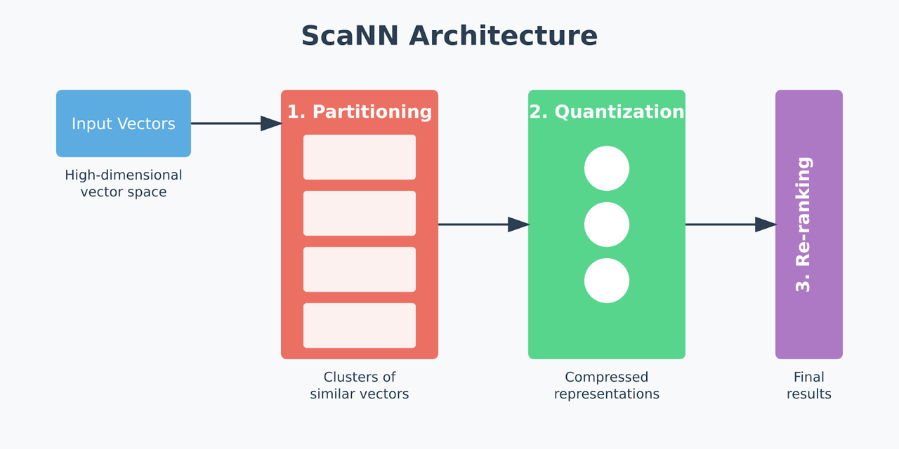
- Partitioning: Divides the dataset into clusters. This method narrows the search space by focusing only on relevant data subsets instead of scanning the entire dataset, saving time and processing resources. ScaNN often uses clustering algorithms, such as k-means, to identify clusters, which allows it to perform similarity searches more efficiently.
- Quantization: ScaNN applies a quantization process known as anisotropic vector quantization after partitioning. Traditional quantization focuses on minimizing the overall distance between original and compressed vectors, which isn't ideal for tasks like Maximum Inner Product Search (MIPS), where similarity is determined by the inner product of vectors rather than direct distance. Anisotropic quantization instead prioritizes preserving parallel components between vectors, or the parts most important for calculating accurate iner products. This approach allows ScaNN to maintain high MIPS accuracy by carefully aligning compressed vectors with the query, enabling faster, more precise similarity searches.
- Re-ranking: The re-ranking phase is the final step, where ScaNN fine-tunes the search results from the partitioning and quantization stages. This re-ranking applies precise inner product calculations to the top candidate vectors, ensuring the final results are highly accurate. Re-ranking is crucial in high-spped recommendation engines or image search applications where the initial filtering and clustering serve as a coarse layer, and the final stage ensures that only the most relevant results are returned to the user.
The performance of SCANN is controlled by two key parameters that let you fine-tune the balance between speed and accuracy:
with_raw_data: Controls whether original vector data is stored alongside quantized representations. Enabling this parameter improves accuracy during re-ranking but increases storage requirements.reorder_k: Determines how many candidates are refined during the final re-ranking phase. Higher values improve accuracy but increase search latency.
For detailed guidance on optimizing these parameters for your specific use case, refer to Index params.
# Build index
To build a SCANN index on a vector field in Milvus, use the add_index() method, specifying the index_type, metric_type, and additional parameters for the index.
from pymilvus import MilvusClient
# Prepare index building params
index_params = MilvusClient.prepare_index_params()
index_params.add_index(
field_name="your_vector_field_name", # Name of the vector field to be indexed
index_type="SCANN", # Type of the index to create
index_name="vector_index", # Name of the index to create
metric_type="L2", # Metric type used to measure similarity
params={
"with_raw_data": True, # Whether to hold raw data
} # Index building params
)
2
3
4
5
6
7
8
9
10
11
12
13
14
In this configuration:
index_type: The type of index to be built. In this example, set the value toSCANN.metric_type: The method used to calculate the distance between vectors. Supported values includeCOSINE,L2, andIP. For details, refer to Metric Types.params: Additional configuration options for building the index.with_raw_data: Whether to store the original vector data alongside the quantized representation.
To learn more building parameters available for the SCANN index, refer to Index building params.
Once the index parameters are configured, you can create the index by using the create_index() method directly or passing the index params in the create_collection method. For details, refer to Create Collection.
# Search on index
Once the index is built and entities are inserted, you can perform similarity searches on the index.
search_params = {
"params": {
"reorder_k": 10, # Number of candidates to refine
}
}
res = MilvusClient.search(
collection_name="your_collection_name", # Collection name
anns_field="vector_field", # Vector field name
data=[[0.1, 0.2, 0.3, 0.4, 0.5]], # Query vector
limit=10, # TopK results to return
search_params=search_params
)
2
3
4
5
6
7
8
9
10
11
12
13
In this configurations:
params: Additional configuration options for searching on the index.reorder_k: Number of candidates to refine during the re-ranking phase.
To learn more search parameters available for the SCANN index, refer to Index-specific search params.
# Index params
This sectoin provides an overview of the parameters used for building an index and performing searches on the index.
# Index building params
The following table lists the parameters that can be configured in params when building an index.
| Parameter | Description | Value Range | Tuning Suggestion |
|---|---|---|---|
with_raw_data | Whether to store the original vector data alongside the quantized representation. When enabled, this allows for more accurate similarity calculations during the reranking phase by using the original vectors instead of quantized approximations. | Type: Boolean Range: True, False Default value: True | Set to True for higher search accuracy and when storage space is not a primary concern. The original vector data enables more precise similarity calculations during re-ranking. Set to False to reduce storage overhead and memory usage, especially for large datasets. However, this may result in slightly lower search accuracy as the re-ranking phase will use quantized vectors. Recommended: Use True for production applications where accuracy is critical. |
# Index-specific search params
The following table lists the parameters that can be configured in search_params.params when searching on the index.
| Parameter | Description | Value Range | Tuning Suggestion |
|---|---|---|---|
reorder_k | Controls the number of candidate vectors that are refined during the re-ranking phase. This parameter determines how many top candidates from the initial partitioning and quantization stages are re-evaluated using more precise similarity calculations. | Type: Integer Range: [1, int_max] Default value: None | A larger reorder_k generally leads to higher search accuracy as more candidates are considered during the final refinement phase. However, this also increases search time due to additional computation. Consider increasing reorder_k when achieving high recall is critical and search speed is less of a concern. A good starting point is 2-5x your desired limit (TopK results to return). Consider decreasing reorder_k to prioritize faster searches, especially in scenarios where a slight reduction in accuracy is acceptable. |
# Binary Vector Indexes
# BIN_IVF_FLAT
The BIN_IVF_FLAT index is a variant of the IVF_FLAT index exclusively for binary embeddings. It enhances query efficiency by first partitioning the vector data into multiple clusters (nlist units) and then comparing the target input vector to the center of each cluster. BIN_IVF_FLAT significantly reduces query time while allowing users to fine-tune the balance between accuracy and speed. For more information, refer to IVF_FLAT.
# Build index
To build a BIN_IVF_FLAT index on a vector field in Milvus, use the add_index() method, specifying the index_type, metric_type, and additional parameters for the index.
from pymilvus import MilvusClient
# Prepare index building params
index_params = MilvusClient.prepare_index_params()
index_params.add_index(
field_name="your_binary_vector_field_name", # Name of the vector field to be indexed
index_type="BIN_IVF_FLAT", # Type of the index to create
index_name="vector_index", # Name of the index to create
metric_type="HAMMING", # Metric type used to measure similarity
params={
"nlist": 64, # Number of clusters for the index
} # Index building params
)
2
3
4
5
6
7
8
9
10
11
12
13
14
In this configuration:
index_type: The type of index to be built. In this example, set the value toBIN_IVF_FLAT.metric_type: The method used to calculate the distance between vectors. Supported values for binary embeddings includeHAMMING(default) andJACCARD. For details, refer to Metric Types.params: Additional configuration options for building the index.nlist: Number of clusters to divide the dataset.
To learn more building parameters available for the BIN_IVF_FLAT index, refer to Index building params.
Once the index parameters are configured, you can create the index by using the create_index() method directly or passing the index params in the create_collection method. For details, refer to Create Collection.
# Search on index
Once the index is built and entities are inserted, you can perform similarity searches on the index.
search_params = {
"params": {
"nprobe": 10, # Number of clusters to search
}
}
res = MilvusClient.search(
collection_name="your_collection_name", # Collection name
anns_field="binary_vector_field", # Binary vector field
data=[query_binary_vector], # Query binary vector
limit=3, # TopK results to return
search_params=search_params
)
2
3
4
5
6
7
8
9
10
11
12
13
In this configuration:
params: Additional configuration options for searching on the index.nprobe: Number of clusters to search for.
To learn more search parameters available for the BIN_IVF_FLAT index, refer to Index-specific search params.
# Index params
This section provides an overview of the parameters used for building an index and performing searches on the index.
# Index building params
The following table lists the parameters that can be configured in params when building an index.
| Parameter | Description | Value Range | Tuning Suggestion |
|---|---|---|---|
nlist | The number of clusters to create using the k-means algorithm during index building. Each cluster, represented by a centroid, sotres a list of vectors. Increasing this parameter reduces the number of vectors in each cluster, creating smaller, more focused partitions. | Type: Integer Range: [1, 65536] Default value: 128 | Larger nlist values improve recall by creating more refined clusters but increase index building time. Optimize based on dataset size and available resources. In most cases, we recommend you set a value within this range: [32, 4096]. |
# Index-specific search params
The following table lists the parameters that can be configured in search_params.param when searching on the index.
| Parameter | Description | Value Range | Tuning Suggestion |
|---|---|---|---|
nprobe | The number of clusters to search for candidates. Higher values allow more clusters to be searched, improving recall by expanding the search scope but at the cost of increased query latency. | Type: Integer Range: [1, nlist] Default value: 8 | Increasing this value improves recall but may slow down the search. Set nprobe proportionally to nlist to balance speed and accuracy. In most cases, we recommend you set a value within this range: [1, nlist]. |
# BIN_FLAT
The BIN_FLAT index is a variant of the FLAT index tailored exclusively for binary embeddings. It excels in applications where vector similarity search demands perfect accuracy on relatively small, million-scale datasets. By employing an exhaustive search methodology--comparing every target input against all vectors in the dataset--BIN_FLAT guarantees exact results. This precision makes it ideal benchmark for assessing the performance of other indexes that might offer less than 100% recall, although its thorough approach also renders it the slowest option for large-scale data.
# Build index
To build a BIN_FLAT index on a vector field in Milvus, use the add_index() method, specifying the index_type and metric_type parameters for the index.
from pymilvus import MilvusClient
# Prepare index building params
index_params = MilvusClient.prepare_index_params()
index_params.add_index(
field_name="your_binary_vector_field_name", # Name of the vector field to be indexed
index_type="BIN_FLAT", # Type of the index to create
index_name="vector_index", # Name of the index to create
metric_type="HAMMING", # Metric type used to measure similarity
params={} # No additional parameters required for BIN_FLAT
)
2
3
4
5
6
7
8
9
10
11
12
In this configuration:
index_type: The type of index to be built. In this example, set the value toBIN_FLAT.metric_type: The method used to calculate the distance between vectors. Supported values for binary embeddings includeHAMMING(default) andJACCARD. For details, refer to Metric Types.params: No extra parameters are needed for the BIN_FLAT index.
Once the index parameters are configured, you can create the index by using the create_index() method directly or passing the index params in the create_collection method. For details, refer to Create Collection.
# Search on index
Once the index is built and entities are inserted, you can perform similarity searches on the index.
res = MilvusClient.search(
collection_name="your_collection_name", # Collection name
anns_field="binary_vector_field", # Binary vector field name
data=[query_binary_vector], # Query binary vector
limit=3, # TopK results to return
search_params={"params": {}} # No additional parameters required for BIN_FLAT
)
2
3
4
5
6
7
For more inforamtion, refer to Binary Vector.
# Index params
For the BIN_FLAT index, no additional parameters are needed either during the index creation or the search process.
# MINHASH_LSH
Efficient deduplication and similarity search are critical for large-scale machine learning datasets, especially for tasks like cleaning training corpora for Large Language Models (LLMs). When dealing with millions or billions of documents, traditional exact matching becomes too slow and costly.
The MINHASH_LSH index in Milvus enables fast, scalable, and accurate approximate deduplication by combining two powerful techniques:
- MinHash: Quickly generates compact signatures (or "fingerprints") to estimate document similarity.
- Locality-Sensitive Hashing (LSH): Rapidly finds group of similar documents based on their MinHash signatures.
This guide walks you through the concepts, prerequisites, setup, and best practices for using MINHASH_LSH in Milvus.
# Overview
# Jaccard similarity
Jaccard similarity measures the overlap between two sets A and B, formally defined as:
J(A,B)=∣A∪B∣∣A∩B∣
Where its value ranges from 0 (completely disjoint) to 1 (identical).
However, computing Jaccard similarity exactly between all document pairs in large-scale datasets is computationally expensive -- O(n2) in time and memory when n is large. This makes it infeasible for use cases such as LLM training corpus cleaning or web-scale document analysis.
# MinHash signatures: Approximate Jaccard similarity
MinHash is a probabilistic technique that offers an efficient way to estimate Jaccard similarity. It works by transforming each set into a compact signature vector, preserving enough information to approximate set similarity efficiently.
The core idea:
The more similar the two sets are, the more likely their MinHash signatures will match at the same positions. This property enables MinHash to approximate the Jaccard similarity between sets.
This property allows MinHash to approximate the Jaccard similarity between sets without needing to compare the full sets directly.
The MinHash process involves:
- Shingling: Convert documents into sets of overlapping token sequences (shingles)
- Hashing: Apply multiple independent hash functions to each shingle
- Min Selection: For each hash function, record the minimum hash value across all shingles
You can see the entire process illustrated below:
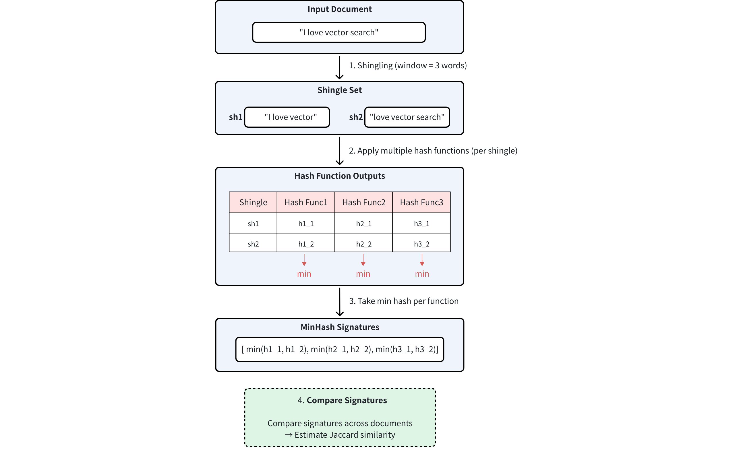
NOTE
The number of hash functions used determines the dimensionality of the MinHash signature. Higher dimensions provide better approximation accuracy, at the cost of increased storage and computation.
# LSH for MinHash
While MinHash signatures significantly reduce the cost of computing exact Jaccard similarity between documents, exhaustively comparing every pair of signature vectors is still inefficient at scale.
To solve this, LSH is used. LSH enables fast approximate similarity search by ensuring that similar items are hashed into the same "bucket" with high probability -- avoiding the need to compare every pair directly.
The process involves:
- Signature segmentation: An n-dimensional MinHash signature is divided into b bands. Each band contains r consecutive hash values, so the total signature length satisfies: n=b×r. For example, if you have a 128-dimensional MinHash signature (n = 128) and divide it into 32 bands (b = 32), then each band contains 4 hash values (r = 4).
- Band-level hashing: After segmentation, each band is independently processed using a standard hash function to assign it to a bucket. If two signatures produce the same hash value within a band -- i.e. they fall into the same bucket -- they are considered potential matches.
- Candidate selection: Pairs that collide in at least one band are selected as similarity candidates.
NOTE
Why it works?
Mathematically, if two signatures have Jaccard similarity s,
- The probability they are identical in one row (hash position) is s
- The probability they match in all r rows of a band is sr
- The probability that they match in at least one band is:
1−(1−sr)b
For details, refer to Locality-sensitive hashing.
Consider three documents with 128-dimensional MinHash signatures:

First, LSH divides the 128-dimensional signature into 32 bands of 4 consecutive values each:

Then, each band is hashed into different buckets using a hash function. Document pairs sharing buckets are selected as similarity candidates. In the example below, Document A and Document B are selected as similarity candidates as their hash results collide in Band 0:
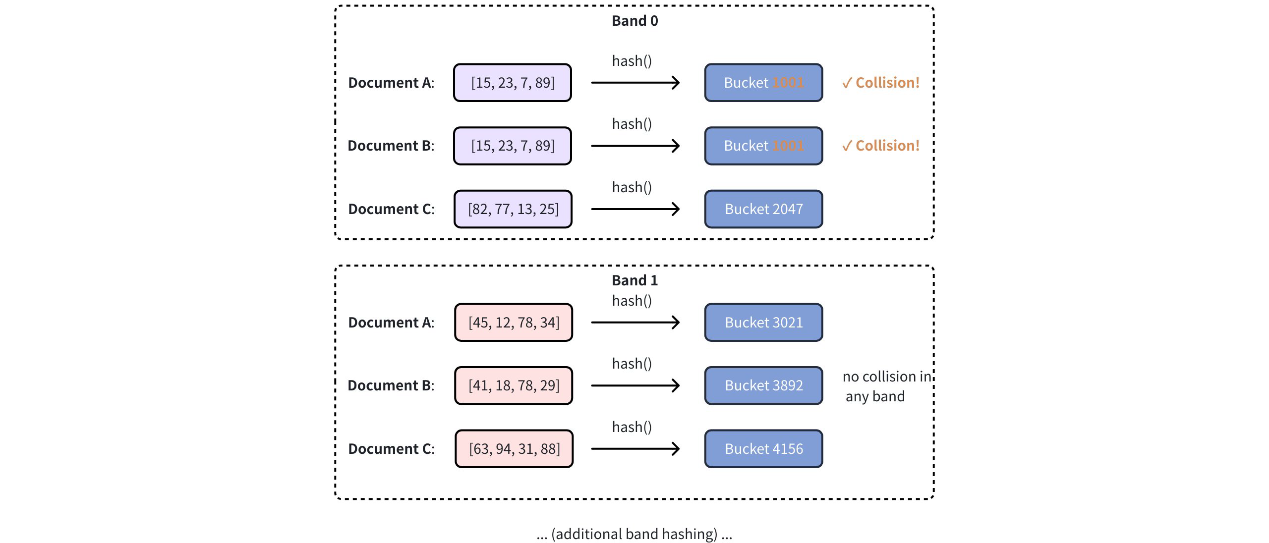
NOTE
The number of bands is controlled by the mh_lsh_band parameter. For more information, refer to Index building params.
# MHJACCARD: Comparing MinHash signatures in Milvus
MinHash signatures approximate the Jaccard similarity between sets using fixed-length binary vectors. However, since these signatures do not preserve the original sets, standard metrics such as JACCARD, L2, or COSINE cannot be directly applied to compare them.
To address this, Milvus introduces a specialized metric type called MHJACCARD, designed specifically for comparing MinHash signatures.
When using MinHash in Milvus:
- The vector field must be of type
BINARY_VECTOR - The
index_typemust beMINHASH_LSH(orBIN_FLAT) - The
metric_typemust be set toMHJACCARD
Using other metrics will either be invalid or yield incorrect results.
For more information about this metric type, refer to MHJACCARD.
# Prerequisites
Before using MinHash LSH in Milvus, you must first generate MinHash signatures. These compact binary signatures approximate Jaccard similarity between sets and are required for MHJACCARD-based search in Milvus.
# Choose a method to generate MinHash signatures
Depending on your workload, you can choose:
- Use Python's
datasketchfor simplicity (recommended for prototyping) - Use distributed tools (e.g., Spark, Ray) for large-scale datasets
- Implement custom logic (Numpy, C++, etc.) if performance tuning is critical
In this guide, we use datasketch for simplicity and compatibility with Milvus input format.
# Install required libraries
Install the necessary packages for this example:
pip install pymilvus datasketch numpy
# Generate MinHash signatures
We'll generate 256-dimensional MinHash signatures, with each hash value represented as a 64-bit integer. This alighs with the expected vector format for MINHASH_LSH.
from datasketch import MinHash
import numpy as np
MINHASH_DIM = 256
HASH_BIT_WIDTH = 64
def generate_minhash_signature(text, num_perm=MINHASH_DIM) -> bytes:
m = MinHash(num_perm=num_perm)
for token in text.lower().split():
m.update(token.encode("utf8"))
return m.hashvalues.astype('>u8').tobytes() # Returns 2048 bytes
2
3
4
5
6
7
8
9
10
11
Each signature is 256 x 64 bites = 2048 bytes. This byte string can be directly inserted into a Milvus BINARY_VECTOR field. For more information on binary vectors used in Milvus, refer to Binary Vector.
# (Optional) Prepare raw token sets (for refined search)
By default, Milvus uses only the MinHash signatures and LSH index to find approximate neighbors. This is fast but may return false positives or miss close matches.
If you want accurate Jaccard similarity, Milvus supports refined search that uses original token sets. To enable it:
- Store token sets as a separate
VARCHARfield - Set
"with_raw_data": Truewhen building index parameters - And enable
"mh_search_with_jaccard": Truewhen performing similarity search
Token set extraction example:
def extract_token_set(text: str) -> str:
tokens = set(text.lower().split())
return " ".join(tokens)
2
3
# Use MinHash LSH in Milvus
Once your MinHash vectors and original token sets are ready, you can store, index, and search them using Milvus with MINHASH_LSH.
# Connect to Milvus
from pymilvus import MilvusClient
client = MilvusClient(uri="http://localhost:19530") # Update if your URI is different
2
3
# Define collection schema
Define a schema with:
- The primary key
- A
BINARY_VECTORfield for the MinHash signatures - A
VARCHARfield for the original token set (if refined search is enabled) - Optionally, a
documentfield for original text
from pymilvus import DataType
VECTOR_DIM = MINHASH_DIM * HASH_BIT_WIDTH
schema = client.create_schema(auto_id=False, enable_dynamic_field=False)
schema.add_field("doc_id", DataType.INT64, is_primary=True)
schema.add_field("minhash_signature", DataType.BINARY_VECTOR, dim=VECTOR_DIM)
schema.add_field("token_set", DataType.VARCHAR, max_length=1000) # required for refinement
schema.add_field("document", DataType.VARCHAR, max_length=1000)
2
3
4
5
6
7
8
9
# Build index parameters and create collection
Build a MINHASH_LSH index with Jaccard refinement enabled:
index_params = client.prepare_index_params()
index_params.add_index(
field_name="minhash_signature",
index_type="MINHASH_LSH",
metric_type="MHJACCARD",
params={
"mh_element_bit_width": HASH_BIT_WIDTH, # Must match signature bit width
"mh_lsh_band": 16, # Band count (128/16 = 8 hashes per band)
"with_raw_data": True # Required for Jaccard refinement
}
)
client.create_collection("minhash_demo", schema=schema, index_params=index_params)
2
3
4
5
6
7
8
9
10
11
12
13
For more information on index building parameters, refer to Index building params.
# Insert data
For each document, prepare:
- A binary MinHash signature
- A serialized token set string
- (Optionally) the original text
documents = [
"machine learning algorithms process data automatically",
"deep learning uses neural networks to model patterns"
]
insert_data = []
for i, doc in enumerate(documents):
sig = generate_minhash_signature(doc)
token_str = extract_token_set(doc)
insert_data.append({
"doc_id": i,
"minhash_signature": sig,
"token_set": token_str,
"document": doc
})
client.insert("minhash_demo", insert_data)
client.flush("minhash_demo")
2
3
4
5
6
7
8
9
10
11
12
13
14
15
16
17
18
# Perform similarity search
Milvus supports two modes of similarity search using MinHash LSH:
- Approximate search: uses only MinHash signatures and LSH for fast but probabilistic results.
- Refined search: re-computes Jaccard similarity using original token sets for improved accuracy.
5.1 Prepare the query: To perform a similarity search, generate a MinHash signature for the query document. This signature must match the same dimension and encoding format used during data insertion.
query_text = "neural networks model patterns in data"
query_sig = generate_minhash_signature(query_text)
2
5.2 Approximate search (LSH-only): This is fast and scalable but may miss close matches or include false positives:
search_params = {
"metric_type": "MHJACCARD",
"params": {}
}
approx_results = client.search(
collection_name="minhash_demo",
data=[query_sig],
anns_field="minhash_signature",
search_params=search_params,
limit=3,
output_fields=["doc_id", "document"],
consistency_level="Bounded"
)
for i, hit in enumerate(approx_results[0]):
sim = 1 - hit['distance']
print(f"{i+1}. Similarity: {sim:.3f} | {hit['entity']['document']}")
2
3
4
5
6
7
8
9
10
11
12
13
14
15
16
17
18
5.3 Refined search (recommended for accuracy): This enable accurate Jaccard comparison using the original token sets stored in Milvus. It's slightly slower but recommended for quality-sensitive tasks:
search_params = {
"metric_type": "MHJACCARD",
"params": {
"mh_search_with_jaccard": True, # Enable real Jaccard computation
"refine_k": 5 # Refine top 5 candidates
}
}
refined_results = client.search(
collection_name="minhash_demo",
data=[query_sig],
anns_field="minhash_signature",
search_params=search_params,
limit=3,
output_fields=["doc_id", "document"],
consistency_level="Bounded"
)
for i, hit in enumerate(refined_results[0]):
sim = 1 - hit['distance']
print(f"{i+1}. Similarity: {sim:.3f} | {hit['entity']['document']}")
2
3
4
5
6
7
8
9
10
11
12
13
14
15
16
17
18
19
20
21
# Index params
This section provides an overview of the parameters used for building an index and performing searches on the index.
# Index building params
The following table lists the parameters that can be configured in params when building an index.
|Parameter|Description|Value Range|Tuning Suggestion|
|||||
|mh_element_bit_width|Bit width of each hash value in the MinHash signature. Must be divisible by 8.|8, 16, 32, 64|Use 32 for balanced performance and accuracy. Use 64 for higher precision with larger datasets. Use 16 to save memory with acceptable accuracy loss.|
|mh_lsh_band|Number of bands to divide the MinHash signature for LSH. Controls the recall performance tradeoff.|[1, signature_length]|For 128-dim signatures: start with 32 bands (4 values/band). Increase for 64 for higher recall, decrease to 16 for better performance. Must divide signature length evenly.|
|mh_lsh_code_in_mem|Whether to store LSH hash codes in anonymous memory (true) or use memory mapping (false).|true, false|Use false for large datasets (>1M sets) to reduce memory usage. Use true for smaller datasets requiring maximum search speed.|
|with_raw_data|Wheter to store original MinHash signatures alongside LSH codes for refinement.|true, false|Use true when high precision is required and storage cost is acceptable. Use false to minimize storage overhead with slight accuracy reduction.|
|mh_lsh_bloom_false_positive_prob|False positive probability for Bloom filter used in LSH bucket optimization.|[0.001, 0.1]|Use 0.01 for balanced memory usage and accuracy. Lower values (0.001) reduce false positives but increase memory. Higher values (0.05) save memory but may reduce precision.|
# Index-specific search params
The following table lists the parameters that can be configured in search_params.params when searching on the index.
| Parameter | Description | Value Range | Tuning Suggestion |
|---|---|---|---|
mh_search_with_jaccard | Wheter to perform exact Jaccard similarity computation on candidate results for refinement. | true, false | Use true for applications requiring high precision (e.g., deduplication). Use false for faster approximate search when slight accuracy loss is acceptable. |
refine_k | Number of candidates to retrieve before Jaccard refinement. Only effective when mh_search_with_jaccard is true | [tok_k, top_k * 10] | set to 2-5x the desired top_k for good recall performance balance. Higher values improve recall but increase computation cost. |
mh_lsh_batch_search | Whether to enable batch optimization for multiple simultaneous queries. | true, false | Use true when searching with multiple queries simultaneously for better throughput. Use false for single-query scenarios to reduce memory overhead. |
# Sparse Vector Indexes
# SPARSE_INVERTED_INDEX
The SPARSE_INVERTED_INDEX index is an index type used by Milvus to efficiently store and sparse vectors. This index type leverages the principles of inverted indexing to create a highly efficient search structure for sparse data. For more information, refer to INVERTED.
# Build index
To build a SPARSE_IVERTED_INDEX index on a sparse vector field in Milvus, use the add_index() method, specifying the index_type, metric_type, and additional parameters for the index.
from pymilvus import MilvusClient
# Prepare index building params
index_params = MilvusClient.prepare_index_params()
index_params.add_index(
field_name="your_sparse_vector_field_name", # Name of the vector field to be indexed
index_type="SPARSE_INVERTED_INDEX", # Type of the index to create
index_name="sparse_inverted_index", # Name of the index to create
metric_type="IP", # Metric type used to measure similarity
params={"inverted_index_algo": "DAAT_MAXSCORE"}, # Algorithm used for building and querying the index
)
2
3
4
5
6
7
8
9
10
11
12
In this configuration:
index_type: The type of index to built. In this example, set the value toSPARSE_INVERTED_INDEX.metric_type: The metric used to calculate similarity between sparse vectors. Valid Values:IP(Inner Product): Measures similarity using dot product.BM25: Typically used for full-text search, focusing on textual similarity. For further details, refer to Metric Types and Full Text Search.
params.inverted_index_algo: The algorithm used for building and querying the index. Valid values:"DAAT_MAXSCORE"(default): Optimized Document-at-a-Time (DAAT) query processing using the MaxScore algorithm. MaxScore provides better performance for high k values or queries with many terms by skipping terms and documents likely to have minimal impact. It achieves this by partitioning terms into essential and nonessential groups based on their maximum impact scores, focusing on terms that can contribute to the top-k results.DAAT_WAND: Optimized DAAT query processing using the WAND algorithm. WAND evaluates fewer hit documents by leveraging maximum impact scores to skip non-competitive documents, but it has a higher per-hit overhead. This makes WAND more efficient for queries with small k values or short queries, where skipping is more feasible.TAAT_NAIVE: Basic Term-at-a-Time (TAAT) query processing. While it is slower compared toDAAT_MAXSCOREandDAAT_WAND,TAAT_NAIVEoffers a unique advantage. Unlike DAAT algorithms, which use cached maximum impact scores that remain static regardless of changes to the global collection parameter (avgdl),TAAT_NAIVEdynamically adapts to such changes.
To learn more building parameters available for the SPARSE_INVERTED_INDEX index, refer to Index building params.
Once the index parameters are configured, you can create the index by using the create_index() method directly or passing the index params in the create_collection method. For details, refer to Create Collection
# Search on index
Once the index is built and entities are inserted, you can perform similarity searches on the index.
# Prepare search parameters
search_params = {
"params": {"drop_ratio_search": 0.2}, # Additional optional search parameters
}
# Prepare the query vector
query_vector = [{1: 0.2, 50: 0.4, 1000: 0.7}]
res = MilvusClient.search(
collection_name="your_collection_name", # Collection name
anns_field="vector_field", # Vector field name
data=query_vector, # Query vector
limit=3, # TopK results to return
search_params=search_params
)
2
3
4
5
6
7
8
9
10
11
12
13
14
15
In this configuration:
params: Additional configuration options for searching on the index.drop_ratio_search: Fine-tunes search performance by specifying what proportion of small vector values to ignore during the search process. For example, with{"drop_ratio_search": 0.2}, the smallest 20% of values in the query vector will be ignored during the search.
To learn more search parameters available for the SPARSE_INVERTED_INDEX index, refer to Index-specific search params.
# Index params
This section provides an overview of the parameters used for building an index and performing searches on the index.
# Index building params
The following table lists the parameters that can be configured in params when building an index.
| Parameter | Description | Value Range | Tuning Suggestion |
|---|---|---|---|
inverted_index_algo | The algorithm used for building and querying the index. It determines how the index processes queries | DAAT_MAXSCORE (default), DAAT_WAND, TAAT_NAIVE | Use "DAAT_MAXSCORE" for scenarios with high k values or queries with many terms, which can benefit from skipping non-competitive documents. Choose "DAAT_WAND" for queries with small k values or short queries to leverage more efficient skipping. Use "TAAT_NAIVE" if dynamic adjustment to collection changes (e.g., avgdl) is required. |
# Index-specific search params
The following table lists the parameters that can be configured in search_params.params when searching on the index.
| Parameter | Description | Value Range | Tuning Suggestion |
|---|---|---|---|
drop_ratio_search | The proportion of the smallest values to ignore during search, helping to reduce noise. | Fraction between 0.0 and 1.0 (e.g., 0.2 ingores the smallest 20% of values) | Tune this parameter based on the sparsity and noise level of your query vectors. For example, setting it to 0.2 can help focus on more significant values during the search, potentially improving accuracy. |
# Scalar Indexes
# BITMAP
Bitmap indexing is an efficient indexing technique designed to improve query performance on low-cardinality scalar fields. Cardinality refers to the number of distinct values in a field. Fields with fewer distinct elements are considered low-cardinality.
This index type helps reduce the retrieval time of scalar queries by representing field values in a compact binary format and performing efficient bitwise operations on them. Compared to other types of indexes, bitmap indexes typically have higher space efficiency and faster query speeds when dealing with low-cardinality fields.
# Overview
The term Bitmap combines two words: Bit and Map. A bit represents the smallest unit of data in a computer, which can only hold a value of either 0 or 1. A map, in this context, refers to the process of transforming and organizing data according to what value should be assigned to 0 and 1.
A bitmap index consists of two main components: bitmaps and keys. Keys represent the unique values in the indexed field. For each unique value, there is a corresponding bitmap. The length of these bitmaps is equal to the number of records in the collection. Each bit in the bitmap corresponds to a record in the collection. If the value of the indexed field in a record matches the key, the corresponding bit is set to 1; otherwise, it is set to 0.
Consider a collection of documents with fields Category and Public. We want to retrieve documents that fall into the Tech category and are open to the Public. In this case, the keys for our bitmap indexes are Tech and Public.
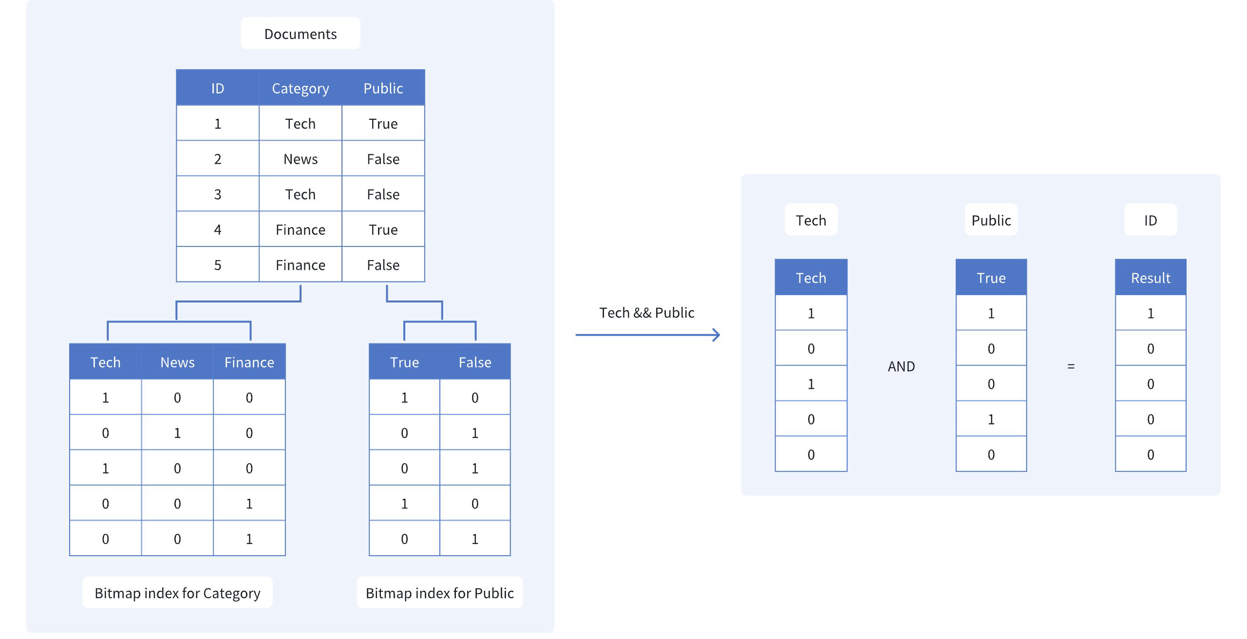
As shown in the figure, the bitmap indexes for Category and Public are:
- Tech: [1, 0, 1, 0, 0], which shows that only the 1st and 3rd documents fall into the Tech category.
- Public: [1, 0, 0, 1, 0], which shows that only the 1st and 4th documents are open to the Public.
To find the documents that match both criteria, we perform a bitwise AND operation on these two bitmaps:
- Tech and Public: [1, 0, 0, 0, 0]
The resulting bitmap [1, 0, 0, 0, 0] indicates that only the first document (ID 1) satisfies both criteria. By using bitmap indexes and efficient bitwise operations, we can quickly narrow down the search scope, eliminating the need to scan the entire dataset.
# Create a bitmap index
To create a bitmap index in Milvus, use the create_index() method and set the index_type parameter to "BITMAP"
from pymilvus import MilvusClient
client = MilvusClient(
uri="http://localhost:19530",
)
index_params = client.create_index_params() # Prepare an empty IndexParams object, without having to specify any index parameters
index_params.add_index(
field_name="category", # Name of the scalar field to be indexed
index_type="BITMAP", # Type of index to be created
index_name="category_bitmap_index" # Name of the index to be created
)
client.create_index(
collection_name="my_collection" , # Specify the collection name
index_params=index_params
)
2
3
4
5
6
7
8
9
10
11
12
13
14
15
16
17
In this example, we create a bitmap index on the category field of the my_collection collection. The add_index method is used to specify the field name, index type, and index name.
Once the bitmap index is created, you can use the filter parameter in query operations to perform scalar filtering based on the indexed field. This allows you to efficiently narrow down the search results using the bitmap index. For more information, refer to Filtering Explained.
# Drop an index
Use the drop_index() method to remove an existing index from a collection.
NOTE
- In v2.6.3 or earlier, you must release the collection before dropping a scalar index.
- From V2.6.4 or later, you can drop a scalar index directly once it's no longer needed -- no need to release the collection first.
client.drop_index(
collection_name="my_collection", # Name of the collection
index_name="category_bitmap_index" # Name of the index to drop
)
2
3
4
# Limits
- Bitmap indexes are supported only for scalar fields that are not primary keys.
- The data type of the field must be one of the following:
BOOL,INT8,INT16,INT32,INT64,VARCHARARRAY(elements must be one of:BOOL,INT8,INT16,INT32,INT64,VARCHAR)
- Bitmap indexes do not support the following data types:
FLOAT,DOUBLE: Floating-point types are not compatible with the binary nature of bitmap indexes.JSON: JSON data types have a complex structure that cannot be efficiently represented using bitmap indexes.
- Bit map indexes are not suitable for fields with high cardinality (i.e., fields with a large number of distinct values).
- As a general guideline, bitmap indexes are most effective when the cardinality of a field is less than 500.
- When the cardinality increases beyond this threshold, the performance benefits of bitmap indexes diminish, and the storage overhead becomes significant.
- For high-cardinality fields, consider using alternative indexing techniques such as inverted indexes, depending on your specific use case and query requirements.
# INVERTED
When you need to perform frequent filter queries on your data, INVERTED indexes can dramatically improve query performance. Instead of scanning through all documents, Milvus uses inverted indexes to quickly locate the exact records that match your filter conditions.
# When to use INVERTED index
Use INVERTED indexes when you need to:
- Filter by specific values: Find all records where a field equals a specific value (e.g.,
category == "electronics") - Filter text content: Perform efficient searches on
VARCHARfields - Query JSON field values: Filter on specific keys within JSON structures
Performance benefit: INVERTED indexes can reduce query time from seconds to milliseconds on large datasets by eliminating the need for full collection scans.
# How INVERTED indexes work
An INVERTED index in Milvus maps each unique field value (term) to the set of document IDs where that value occurs. This structure enables fast lookups for fields with repeated or categorical values.
As shown in the diagram, the process works in two steps:
- Forward mapping (ID -> Term): Each document ID points to the field value it contains.
- Inverted mapping (Term -> IDs): Milvus collects unique terms and builds a reverse mapping from each term to all IDs that contain it.
For example, the value "electronics" maps to IDs 1 and 3, while "books" maps to IDs 2 and 5.

When you filter for a specific value (e.g., category == "electronics"), Milvus simply looks up the term in the index and retrieves the matching IDs directly. This avoids scanning the full dataset and enables fast filtering, especially for categorical or repeated values.
INVERTED indexs suport all scalar field types, such as BOOL, INT8, INT16, INT32, INT64, FLOAT, DOUBLE, DOUBLE, VARCHAR, JSON, and ARRAY. However, the index parameters for indexing a JSON field are slightly different from regular scalar fields.
# Create indexes on non-JSON fields
To create an index on a non-JSON field, follow these steps:
- Prepare your index parameters
from pymilvus import MilvusClient
client = MilvusClient(uri="http://localhost:19530") # Replace with your server address
# Create an empty index parameter object
index_params = client.prepare_index_params()
2
3
4
5
6
- Add the
INVERTEDindex
index_params.add_index(
field_name="category", # Name of the field to index
index_type="INVERTED", # Specify INVERTED index type
index_name="category_index" # Give your index a name
)
2
3
4
5
- Create the index
client.create_index(
collection_name="my_collection", # Replace with your collection name
index_params=index_params
)
2
3
4
# Create indexs on JSON fields
You can also create INVERTED indexes on specific paths with JSON fields. This requires additional parameters to specify the JSON path and data type:
# Build index params
index_params.add_index(
field_name="metadata", # JSON field name
index_type="INVERTED",
index_name="metadata_category_index",
params={
"json_path": "metadata[\"category\"]", # Path to the JSON key
"json_cast_type": "varchar" # Data type to cast to during indexing
}
)
# Create index
client.create_index(
collection_name="my_collection", # Replace with your collection name
index_params=index_params
)
2
3
4
5
6
7
8
9
10
11
12
13
14
15
16
For detailed information about JSON indexing, including supported paths, data types, and limitations, refer to JSON Indexing.
# Drop an index
Use the drop_index() method to remove an existing index from a collection.
NOTE
- In v2.6.3 or earlier, you must release the collection before dropping a scalar index.
- From v2.6.4 or later, you can drop a scalar index directly once it's no longer needed -- no need to release the collection first.
client.drop_index(
collection_name="my_collection", # Name of the collection
index_name="category_index" # Name of the index to drop
)
2
3
4
# Best practices
- Create indexes after loading data: Build indexes on collections that already contain data for better performance
- Use descriptive index names: Choose names that clearly indicate the field and purpose
- Monitor index performance: Check query performance before and after creating indexes
- Consider your query patterns: Create indexes on fields you frequently filter by
# NGRAM
The NGRAM index in Milvus is built to accelerate LIKE queries on VARCHAR fields or specific JSOn paths within JSON fields. Before building the index, Milvus splits text into short, overlapping substrings of a fixed length n, known as n-grams. For example, witn n = 3, the word "Milvus" is split into 3-grams: "Mil", "ilv", "lvu", and "vus". These n-grams are then stored in an inverted index that maps each gram to the document IDs in which it appears. At query time, this index allows Milvus to quickly narrow the search to a small set of candidates, resulting in much faster query execution.
Use it when you need fast prefix, suffix, infix, or wildcard filtering such as:
name LIKE "data%"title LIKE "%vector%"path LIKE "%json"
NOTE
For details on filter expression syntax, refer to Basic Operators.
# How it works
Milvus implements the NGRAM index in a two-phase process:
- Build index: Generate n-grams for each document and build an inverted index during ingest.
- Accelerate queries: Use the index to filter to a small candidate set, then verify exact matches.
# Phase 1: Build the index
During data ingestion, Milvus builds the NGRAM index by performing two main steps:
Decompose text into n-grams: Milvus slides a window of n across each string in the target field and extracts overlapping substrings, or n-grams. The length of these substrings falls within a configurable range,
[min_gram, max_gram].min_gram: The shortest n-gram to generate. This also defines the minimum query substring length that can benefit from the index.max_gram: The longest n-gram to generate. At query time, it is also used as the maximum window size when splitting long query strings.
For example, with
min_gram=2andmax_gram=3, the string"AI database"is broken down as follows:- 2-grams:
AI,I_,_d,da,at, ... - 3-grams:
AI_,I_d,_da,dat,ata, ...

Note
- For a range
[min_gram, max_gram], Milvus generates all n-grams for every length between the two values (inclusive). Example: with[2, 4]and the word"text", Milvus generates:- 2-grams:
te,ex,xt - 3-grams:
tex,ext - 4-grams:
text
- 2-grams:
- N-gram decomposition is character-based and language-agnostic. For example, in Chinese,
"向量数据库"withmin_gram = 2is decomposed into:向量,量数,数据,据库. - Spaces and punctuation are treated as character during decomposition.
- Decomposition preserves original case, and matching is case-sensitive. For example,
"Database"and"database"will generate different n-grams and require exact case matching during queries.
Build an inverted index: An inverted index is created that maps each generated n-gram to a list of the document IDs containing it. For instance, if the 2-gram
"AI"appears in documents with IDs, 1, 5, 6, 8, and 9, the index records{"AI": [1, 5, 6, 8, 9]}. This index is then used at query time to quickly narrow the search scope.
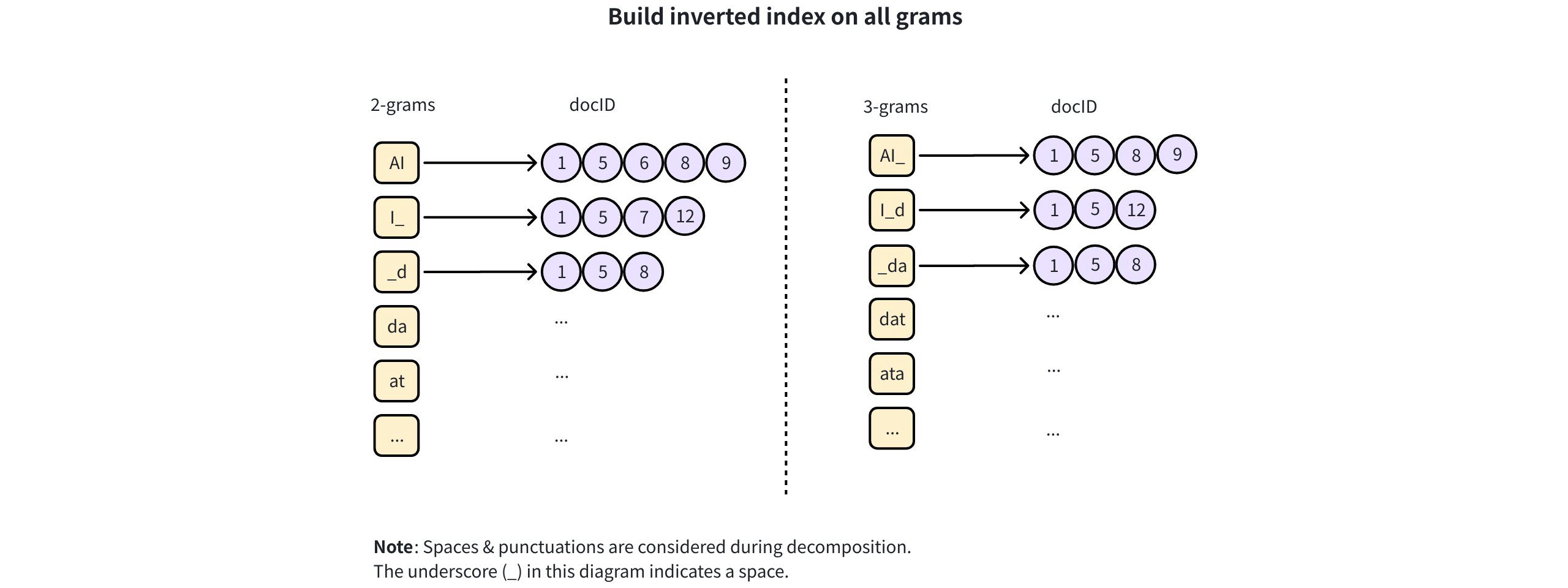
NOTE
A wider [min_gram, max_gram] range creates more grams and larger mapping lists. If memory is tight, consider mmap mode for very large posting lists. For details, refer to Use mmap.
# Phase 2: Accelerate queries
When a LIKE filter is executed, Milvus uses the NGRAM index to accelerate the query in the following steps:
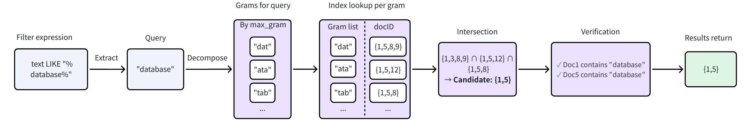
Extract the query term: The contiguous substring without wildcards is extracted from the
LIKEexpression (e.g.,"%database%"becomes"database").Decompose the query term: The query term is decomposed into n-grams based on its length (
L) and themin_gramandmax_gramsettings.- If
L < min_gram, the index cannot be used, and the query falls back to a full scan. - If
min_gram <= L <= max_gram, the entire query term is treated as a single n-gram, and no further decomposition is necessary. - If
L > max_gram, the query term is broken down into overlapping grams using a window size equal tomax_gram.
For example, if the
max_gramis set to3and the query term is"database", which has a length of 8, it is decomposed into 3-gram substrings like"dat",ata,tab, and so on.- If
Look for each gram & intersect: Milvus looks up each of the query grams in the inverted index and then intersects the resulting document ID lists to find a small set of candidate documents. These candidates contain all the grams from the query.
Verify and return results: The original
LIKEfilter is then applied as a final check on only the small candidate set to find the exact matches.
# Create an NGRAM index
You can create an NGRAM index on a VARCHAR field on a specific path inside a JSON field.
# Example 1: Create on a VARCHAR field
For a VARCHAR field, you simply specify the field_name and configure min_gram and max_gram.
from pymilvus import MilvusClient
client = MilvusClient(uri="http://localhost:19530") # Replace with your server address
# Assume you have defined a VARCHAR field named "text" in your collection schema
# Prepare index parameters
index_params = client.prepare_index_params()
# Add NGRAM index on the "text" field
index_params.add_index(
field_name="text", # Target VARCHAR field
index_type="NGRAM", # Index type is NGRAM
index_name="ngram_index", # Custom name for the index
min_gram=2, # Minimum substring length (e.g., 2-gram: "st")
max_gram=3, # Maximum substring length (e.g., 3-gram: "sta")
)
# Create the index on the collection
client.create_index(
collection_name="Documents",
index_params=index_params
)
2
3
4
5
6
7
8
9
10
11
12
13
14
15
16
17
18
19
20
21
22
23
This configuration generates 2-grams and 3-grams for each string in text and stores them in the inverted index.
# Example 2: Create on a JSON path
For a JSON field, in addition to the gram settings, you must also specify:
params.json_path: The JSON path that points to the value you want to index.params.json_cast_type: must be"varchar"(case-insensitive), because NGRAM indexing operates on strings.
# Assume you have defined a JSON field named "json_field" in your collection schema, with a JSON path named "body"
# Prepare index parameters
index_params = client.prepare_index_params()
# Add NGRAM index on a JSON field
index_params.add_index(
field_name="json_field", # Target JSON field
index_type="NGRAM", # Index type is NGRAM
index_name="json_ngram_index", # Custom index name
min_gram=2, # Minimum n-gram length
max_gram=4, # Maximum n-gram length
params={
"json_path": "json_field[\"body\"]", # Path to the value inside the JSON field
"json_cast_type": "varchar" # Required: cast the value to varchar
}
)
# Create the index on the collection
client.create_index(
collection_name="Documents",
index_params=index_params
)
2
3
4
5
6
7
8
9
10
11
12
13
14
15
16
17
18
19
20
21
22
23
In this example:
- Only the value at
json_field["body"]is indexed. - The value is cast to
VARCHARbefore n-gram tokenization. - Milvus generates substrings of length 2 to 4 and stores them in the inverted index.
For more information on how to index a JSON field, refer to JSON Indexing.
# Queries accelerated by NGRAM
For the NGRAM index to be applied:
- The query must target a
VARCHARfield (or JSON path) that has anNGRAMindex. - The literal part of the
LIKEpattern must be at leastmin_gramcharacters long. (For example, if your shortest expected query term is 2 characters, set min_gram=2 when creating the index).
Supported query types:
- Prefix match:
# Match any string that starts with the substring "database"
filter = 'text LIKE "database%"'
2
- Suffix match:
# Match any string that ends with the substring "database"
filter = 'text LIKE "%database"'
2
- Infix match:
# Match any string that contains the substring "database" anywhere
filter = 'text LIKE "%database%"'
2
- Wildcard match:
# Match any string where "st" appears first, and "um" appears later in the text
filter = 'text LIKE "%stu%um%"'
2
- JSON path queries:
filter = 'json_field["body"] LIKE "%database%"'
For more information on filter expression syntax, refer to Basic Operators.
# Drop an index
Use the drop_index() method to remove an existing index from a collection.
NOTE
- In v2.6.3 or ealier, you must release the collection before dropping a scalar index.
- From v2.6.4 or later, you can drop a scalar index directly once it's no longer needed -- no need to release the collection first.
client.drop_index(
collection_name="Documents", # Name of the collection
index_name="ngram_index" # Name of the index to drop
)
2
3
4
# Usage notes
- Field types: Supported on
VARCHARandJSONfields. For JSON, provide bothparams.json_pathandparams.json_cast_type="varchar". - Unicode: NGRAM decomposition is character-based and language-agnostic and includes whitespace and punctuation.
- Space-time trade-off: Wider gram ranges
[min_gram, max_gram]produce more grams and larger indexes. If memory is tight, considermmapmode for large posting lists. For more information, refer to Use mmap. - Immutability:
min_gramandmax_gramcannot be changed in place -- rebuild the index to adjust them.
# Best practices
- Choose min_gram and max_gram to match search behavior:
- Start with
min_gram=2,max_gram=3. - Set
min_gramto the shortest literal you expect users to type. - Set
max_gramnear the typical length of meaningful substrings; largermin_gramimproves filtering but increases space.
- Start with
- Avoid low-selectivity grams: Highly repetitive patterns (e.g.,
"aaaaaa") provide weak filtering and may yield limited gains. - Normalize consistently: Apply the same normalization to ingested text and query literals (e.g., lowercasing, trimming) if your use case needs it.
# RTREE
The RTREE index is a tree-based data structure that accelerates queries on GEOMETRY fields in Milvus. If your collection stores geometric objects such as points, lines, or polygans in Well-known text (WKT) format and you want to accelerate spatial filtering, RTREE is an ideal choice.
# How it works
Milvus uses an RTREE index to efficiently organize and filter geometry data, following a two-phase process:
# Phase 1: Build the index
- Create leaf nodes: For each geometry object, calculate its Minimum Bounding Rectangle (MBR), which is the smallest rectangle that fully contains the object, and store it as a leaf node.
- Group into larger boxes: Cluster nearby leaf nodes together and wrap each group with a new MBR, forming internal nodes. For example, group B contains D and E; group C contains F and G.
- Add the root node: Add a root node whose MBR covers all internal groups, resulting in a height-balanced tree structure.
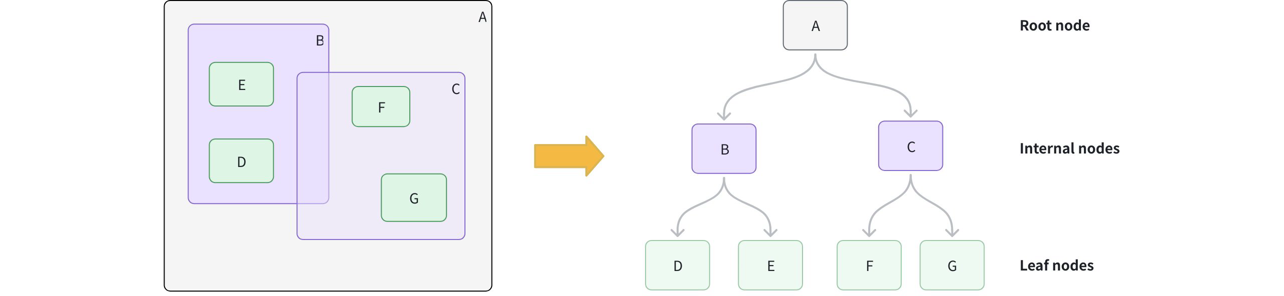
# Phase 2: Accelerate queries
- Form the query MBR: Calculate the MBR for your query geometry.
- Prune branches: Starting at the root, compare the query MBR to each internal node. Skip any branches whose MBR does not intersect with the query MBR.
- Collect candidates: Descend into intersecting branches to gather candidate leaf nodes.
- Exact match: For each candidate, perform an exact spatial predicate to determine true matches.
# Create an RTREE index
You can create an RTREE index on a GEOMETRY field defined in your collection schema.
from pymilvus import MilvusClient
client = MilvusClient(uri="http://localhost:19530") # Replace with your server address
# Assume you have defined a GEOMETRY field named "geo" in your collection schema
# Prepare index parameters
index_params = client.prepare_index_params()
# Add RTREE index on the "geo" field
index_params.add_index(
field_name="geo",
index_type="RTREE", # Spatial index for GEOMETRY
index_name="rtree_geo", # Optional, name your index
params={} # No extra params needed
)
# Create the index on the collection
client.create_index(
collection_name="geo_demo",
index_params=index_params
)
2
3
4
5
6
7
8
9
10
11
12
13
14
15
16
17
18
19
20
21
22
# Query with RTREE
You filter with geometry operators in the filter expression. When an RTREE exists on the target GEOMETRY field, Milvus uses it to prune candidates automatically. Without the index, the filter falls back to a full scan.
For a full list of available geometry-specific operators, refer to Geometry Operators.
# Example 1: Filter only
Find all geometric objects within a given polygon:
filter_expr = "ST_CONTAINS(geo, 'POLYGON((0 0, 10 0, 10 10, 0 10, 0 0))')"
res = client.query(
collection_name="geo_demo",
filter=filter_expr,
output_fields=["id", "geo"],
limit=10
)
print(res) # Expected: a list of rows where geo is entirely inside the polygon
2
3
4
5
6
7
8
9
# Example 2: Vector search + spatial filter
Find the nearest vectors that also intersect a line:
# Assume you've also created an index on "vec" and loaded the collection.
query_vec = [[0.1, 0.2, 0.3, 0.4, 0.5]]
filter_expr = "ST_INTERSECTS(geo, 'LINESTRING(1 1, 2 2)')"
hits = client.search(
collection_name="geo_demo",
data=query_vec,
limit=5,
filter=filter_expr,
output_fields=["id", "geo"]
)
print(hits) # Expected: top-k by vector similarity among rows whose geo intersects the line
2
3
4
5
6
7
8
9
10
11
12
For more information on how to use a GEOMETRY field, refer to Geometry Field.
# Drop an index
Use the drop_index() method to remove an existing index from a collection.
NOTE
- In v2.6.3 or earlier, you must release the collection before dropping a scalar index.
- From v2.6.4 or later, you can drop a scalar index directly once it's no longer needed -- no need to release the collection first.
client.drop_index(
collection_name="geo_demo", # Name of the collection
index_name="rtree_geo" # Name of the index to drop
)
2
3
4
# GPU-enabled Indexes
# GPU Index Overview
Building an index with GPU support in Milvus can significantly improve search performance in high-throughout and high recall scenarios.
The following figure compares the query throughput (queries per second) of various index configurations across different hardware setups, vector datasets (Cohere and OpenAI), and search batch sizes, showing that GPU_CAGRA consistently outperforms other methods.
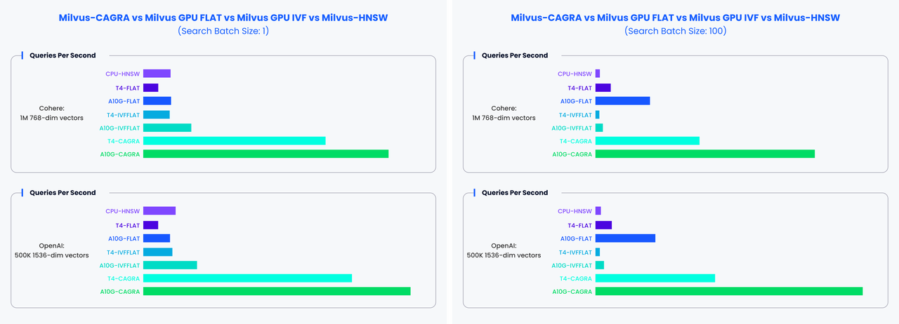
# Limits
- For
GPU_IVF_FLAT, the maximum value forlimitis 1024. - For
GPU_IVF_PQandGPU_CAGRA, the maximum value forlimitis 1024. - While there is no set
limitforGPU_BRUTE_FORCE, it is recommended not to exceed 4096 to avoid potential performance issues. - Currently, GPU indexes do not support
COSINEdistance. IfCOSINEdistance is required, data should be normalized first, and then inner product(IP) distance can be used as a substitute. - Loading OOM protection for GPU indexes is not fully supported, too much data might lead to QueryNode crashes.
- GPU indexes do not support search functions like range search and grouping search.
# Supported GPU index types
The following table lists the GPU index types supported by Mivlus.
| Index Type | Description | Memory Usage |
|---|---|---|
| GPU_CAGRA | GPU_CAGRA is a graph-based index optimized for GPUs, Using inference-grade GPUs to run the Milvus GPU version can be more cost-effective compared to using expensive training-grade GPUs. | Memory usage is approximately 1.8 times that of the original vector data. |
| GPU_IVF_FLAT | GPU_IVF_FLAT is the most basic IVF index, and the encoded data stored in each unit is consistent with the original data. When conducting searches, note that you can set the top-k (limit) up to 256 for any search against a GPU_IVF_FLAT indexed collection. | Requires memory equal to the size of the original data. |
| GPU_IVF_PQ | GPU_IVF_PQ performs IVF index clustering before quantizing the product of vectors. When conducting searches, note that you can set the top-k (limit) up to 8192 for any search against a GPU_IVF_FLAT indexed collection. | Utilizes a smaller memory footprint, which depends on the compression parameter settings. |
| GPU_BRUTE_FORCE | GPU_BRUTE_FORCE is tailored for cases where extremely high recall is crucial, guaranteeing a recall of 1 by comparing each query with all vectors in the dataset. It only requires the metric type (metric_type) and top-k (limit) as index building and search parameters. | Requires memory equal to the size of the original data. |
# Configure Milvus settings for GPU memory control
Milvus uses a global graphics memory pool to allocate GPU memory. It supports two parameters initMemSize and maxMemSize in Milvus config file. The pool size is initially set to initMemSize, and will be automatically expanded to maxMemSize after exceeding this limit.
The default initMemSize is 1/2 of the available GPU memory when Milvus starts, and the default maxMemSize is equal to all avaliable GPU memory.
Up until Milvus 2.4.1, Milvus uses a unified GPU memory pool. For versions prior to 2.4.1, it was recommended to set both of the value to 0.
gpu:
initMemSize: 0 # set the initial memory pool size.
maxMemSize: 0 # maxMemSize sets the maximum memory usage limit.
# When the memory usage exceed initMemSize, Milvus will attempt to expand the memory pool.
2
3
4
From Milvus 2.4.1 onwards, the GPU memory pool is only used for temporary GPU data during searches. Therefore, it is recommended to set it to 2048 and 4096.
gpu:
initMemSize: 2048 # set the initial memory pool size.
maxMemSize: 4096 # maxMemSize sets the maximum memory usage limit.
# When the memory usage exceed initMemSize, Milvus will attempt to expand the memory pool.
2
3
4
To learn how to build a GPU index, refer to the specific guide for each index type.
# FAQ
- When is it appropriate to utilize a GPU index?
A GPU index is particularly beneficial in situations that demand high throughput or high recall. For instance, when dealing with large batches, the throughput of GPU indexing can surpass that of CPU indexing by as much as 100 times. In scenarios with smaller batches, GPU indexing still significantly outshine CPU indexes in terms of performance. Furthermore, if there's a requirement for rapid data insertion, incorporating a GPU can substantially speed up the process of building indexes.
- In which scenarios are GPU indexes like GPU_CAGRA, GPU_IVF_PQ, GPU_IVF_FLAT, and GPU_BRUTE_FORCE most suitable?
GPU_CAGRA indexes are ideal for scenarios that demand enhanced performance, albeit at the cost of consuming more memory. For environments where memory conservation is a priority, the GPU_IVF_PQ index can help minimize storage requirements, though this comes with a higher loss in precision. The GPU_IVF_FLAT index serves as a balanced option, offering a compromise between performance and memory usage. Lastly, the GPU_BRUTE_FORCE index is designed for exhaustive search operations, guaranteeing a recall rate of 1 by performing traversal searches.
# GPU_CAGRA
The GPU_CAGRA index is a graph-based index optimized for GPUs. Using inference-grade GPUs to run the Milvus GPU version can be more cost-effective compared to using expensive training-grade GPUs.
# Build index
To build a GPU_CAGRA index on a vector field in Milvus, use the add_index() method, specifying the index_type, metric_type, and additional parameters for the index.
from pymilvus import MilvusClient
# Prepare index building params
index_params = MilvusClient.prepare_index_params()
index_params.add_index(
field_name="your_vector_field_name", # Name of the vector field to be indexed
index_type="GPU_CAGRA", # Type of the index to create
index_name="vector_index", # Name of the index to create
metric_type="L2", # Metric type used to measure similarity
params={
"intermediate_graph_degree": 64, # Affects recall and build time by determining the graph's degree before pruning
"graph_degree": 32, # Affects search performance and recall by setting the graph's degree after pruning
"build_algo": "IVF_PQ", # Selects the graph generation algorithm before pruning
"cache_dataset_on_device": "true", # Decides whether to cache the original dataset in GPU memory
"adapt_for_cpu": "false", # Decides whether to use GPU for index-building and CPU for search
} # Index building params
)
2
3
4
5
6
7
8
9
10
11
12
13
14
15
16
17
18
In this configuration:
index_type: The type of index to be built. In this example, set the value toGPU_CAGRA.metric_type: The method used to calculate the distance between vectors. For details, refer to Metric Types.params: Additional configuration options for building the index. To learn more building parameters available for theGPU_CAGRAindex, refer to Index building params.
Once the index parameters are configured, you can create the index by using the create_index() method directly or passing the index params in the create_collection method. For details, refer to Create Collection.
# Search on index
Once the index is built and entities are inserted, you can perform similarity searches on the index.
search_params = {
"params": {
"itopk_size": 16, # Determines the size of intermediate results kept during the search
"search_width": 8, # Specifies the number of entry points into the CAGRA graph during the search
}
}
res = MilvusClient.search(
collection_name="your_collection_name", # Collection name
anns_field="vector_field", # Vector field name
data=[[0.1, 0.2, 0.3, 0.4, 0.5]], # Query vector
limit=3, # TopK results to return
search_params=search_params
)
2
3
4
5
6
7
8
9
10
11
12
13
14
In this configuration:
params: Additional configuration options for searching on the index. To learn more search parameters available for theGPU_CAGRAindex, refer to Index-specific search params.
# Enable CPU search at load time
To enable CPU search dynamically at load time, edit the following config in milvus.yaml:
# milvus.yaml
knowhere:
GPU_CAGRA:
load:
adapt_for_cpu: true
2
3
4
5
Behavior:
- When
load.adapt_for_cpuis set totrue, Milvus converts the GPU_CAGRA index into a CPU-executable format (HNSW-like) during load. - Subsequent search operations are executed on CPU, even if the index was originally built for GPU.
- If omitted or false, the index stays on GPU and searches run on GPU.
NOTE
Use load-time CPU adaptation in hybrid or cost-sensitive environments where GPU resources are reserved for index building but searches run on CPU.
# Index params
This section provides an overview of the parameters used for building an index and performing searches on the index.
# Index building params
The following table lists the parameters that can be configured in params when building an index.
| Parameter | Description | Default Value |
|---|---|---|
intermediate_graph_degree | Affects recall and build time by determining the graph's degree before pruning. Recommended values are 32 or 64 | 128 |
graph_degree | Affectrs search performance and recall by setting the graph's degree after pruning. A larger difference between these two degrees results in a longer build time. Its value must be smaller than the value of intermediate_graph_degree. | 64 |
build_algo | Selects the graph generation algorithm before pruning. Possible values: IVF_PQ--Offers higher quality but slower build time. NN_DESCENT--Provides a quicker build with potentially lower recall. | IVF_PQ |
cache_dataset_on_device | Decides whether to cache the original dataset in GPU memory. Possible values: "true"--Caches the original dataset to enhance recall by refining search results. "false"--Does not cache the original dataset to save gpu memory. | "false" |
adapt_for_cpu | Decides whether to use GPU for index-building and CPU for search. Setting this parameter to "true" requires the presence of the ef parameter in the search requests. | "false" |
# Index-specific search params
The following table lists the parameters that can be configured in search_params.params when searching on the index.
| Parameter | Description | Default Value |
|---|---|---|
itopk_size | Determines the size of intermediate results kept during the search. A larger value may improved recall at the expense of search performance. It should be at least equal to the final top-k (limit) value and is typically a power of 2 (e.g., 16, 32, 64, 128). | Empty |
search_width | Specifies the number of entry points into the CAGRA graph during the search. Increasing this value can enhance recall but may impact search performance (e.g. 1, 2, 4, 8, 16, 32) | Empty |
min_iterations/max_iterations | Controls the search iteration process. By default, they are set to 0, and CAGRA automatically determines the number of iterations based on itopk_size and search_width. Adjusting these values manually can help balance performance and accuracy. | 0 |
team_size | Specifies the number of CUDA threads used for calculating metric distance on the GPU. Common values are a power of 2 up to 32 (e.g., 2, 4, 8, 16, 32). It has a minor impact on search performance. The default value is 0, where Milvus automatically selects the team_size based on the vector dimension. | 0 |
ef | Specifies the query time/accuracy trade-off. A higher ef value leads to more accurate but slower search. This parameter is mandatory if you set adapt_for_cpu to true when you build the index. | [top_k, int_max] |
# GPU_IVF_FLAT
The GPU_IVF_FLAT index is a GPU-accelerated version of the IVF_FLAT index, designed exclusively for GPU environments. It partitions vector data into nlist cluster units and computes similarity by first comparing the target query vector with the center of each cluster. By tuning the nprobe parameter, only the most promising clusters are searched, which reduces query time while maintaining a balance between accuracy and speed. For more information on foundational concepts, refer to IVF_FLAT.
# Build index
To build a GPU_IVF_FLAT index on a vector field in Milvus, use the add_index() method, specifying the index_type, metric_type, and additional parameters for the index.
from pymilvus import MilvusClient
# Prepare index building params
index_params = MilvusClient.prepare_index_params()
index_params.add_index(
field_name="your_vector_field_name", # Name of the vector field to be indexed
index_type="GPU_IVF_FLAT", # Type of the index to create
index_name="vector_index", # Name of the index to create
metric_type="L2", # Metric type used to measure similarity
params={
"nlist": 1024, # Number of clusters for the index
} # Index building params
)
2
3
4
5
6
7
8
9
10
11
12
13
14
In this configuration:
index_type: The type of index to be built. In this example, set the value toGPU_IVF_FLAT.metric_type: The method used to calculate the distance between vectors. For details, refer to Metric Types.params: Additional configuration options for building the index.nlist: Number of clusters to divide the dataset.
To learn more building parameters available for the
GPU_IVF_FLATindex, refer to Index building params.
Once the index parameters are configured, you can create the index by using the create_index() method directly or passing the index params in the create_collection method. For details, refer to Create Collection.
# Search on index
Once the index is built and entities are inserted, you can perform similarity searches on the index.
search_params = {
"params": {
"nprobe": 10, # Number of clusters to search
}
}
res = MilvusClient.search(
collection_name="your_collection_name", # Collection name
anns_field="vector_field",
data=[[0.1, 0.2, 0.3, 0.4, 0.5]], # Query vector
limit=3, # TopK results to return
search_params=search_params
)
2
3
4
5
6
7
8
9
10
11
12
13
In this configuration:
params: Additional configuration options for searching on the index.nprobe: Number of clusters to search for.
To learn more search parameters available for the
GPU_IVF_FLATindex, refer to Index-specific search params.
# Index params
This section provides an overview of the parameters used for building an index and performing searches on the index.
# Index building params
The following table lists the parameters that can be configured in params when building an index.
| Parameter | Description | Value Range | Tuning Suggestion |
|---|---|---|---|
nlist | The number of clusters to create using the k-means algorithm during index building. Each cluster, represented by a centroid, stores a list of vectors. Increasing this parameter reduces the number of vectors in each cluster, creating smaller, more focused partitions. | Type: Integer Range: [1, 65536] Default value: 128 | Larger nlist values improve recall by creating more refined clusters but increase index building time. Optimize based on dataset size and available resources. In most cases, we recommend you set a value within this range: [32, 4096]. |
# Index-specific search params
The following table lists the parameters that can be configured in search_params.params when searching on the index.
| Parameter | Description | Value Range | Tuning Suggestion |
|---|---|---|---|
nprobe | The number of clusters to search for candidates. Higher values allow more clusters to be searched, improving recall by expanding the search scope but at the cost of increased query latency. | Type: Integer Range: [1, nlist] Default value: 8 | Increasing this value improves recall but may slow down the search. Set nprobe proportionally to nlist to balance speed and accuracy. In most cases, we recommend you set a value within this range: [1, nlist]. |
# GPU_IVF_PQ
The GPU_IVF_PQ index builds on the IVF_PQ concept by combining inverted file clustering with Product Quantization (PQ), which breaks down high-dimensional vectors into smaller subspaces and quantizes them for efficient similarity searches. Exclusively designed for GPU environments, GPU_IVF_PQ leverages parallel processing to accelerate computations and handle large-scale vector data effectively. For more information on foundational concepts, refer to IVF_PQ.
# Build index
To build a GPU_IVF_PQ index on a vector field in Milvus, use the add_index() method, specifying the index_type, metric_type, and additional parameters for the index.
from pymilvus import MilvusClient
# Prepare index building params
index_params = MilvusClient.prepare_index_params()
index_params.add_index(
field_name="your_vector_field_name", # Name of the vector field to be indexed
index_type="GPU_IVF_PQ", # Type of the index to create
index_name="vector_index", # Name of the index to create
metric_type="L2", # Metric type used to measure similarity
params={
"m": 4, # Number of sub-vectors to split each vector into
} # Index building params
)
2
3
4
5
6
7
8
9
10
11
12
13
14
In this configuration:
index_type: The type of index to be built. In this example, set the value toGPU_IVF_PQ.metric_type: The method used to calculate the distance between vectors. Supported values includeCOSINE,L2, andIP. For details, refer to Metric Types.params: Additional configuration options for building the index.m: Number of sub-vectors to split the vector into.
To learn more building parameters available for the GPU_IVF_PQ index, refer to Index building params.
Once the index parameters are configured, you can create the index by using the create_index() method directly or passing the index params in the create_collection method. For details, refer to Create Collection.
# Search on index
Once the index is built and entities are inserted, you can perform similarity searches on the index.
search_params = {
"params": {
"nprobe": 10, # Number of clusters to search
}
}
res = MilvusClient.search(
collection_name="your_collection_name", # Collection name
anns_field="vector_field", # Vector field name
data=[[0.1, 0.2, 0.3, 0.4, 0.5]], # Query vector
limit=3, # TopK results to return
search_params=search_params
)
2
3
4
5
6
7
8
9
10
11
12
13
In this configuration:
params: Additional configuration options for searching on the index.nprobe: Number of clusters to search for.
# Index params
This section provides an overview of the parameters used for building an index and performing searches on the index.
# Index building params
The following table lists the parameters that can be configured in params when building an index.
| Index | Parameter | Description | Value Range | Tuning Suggestion |
|---|---|---|---|---|
| IVF | nlist | The number of clusters to create using the k-means algorithm during index building. | Type: Integer Range: [1, 65536] Default value: 128 | Larger nlist values improve recall by creating more refined clusters but increase index building time. Optimize based on dataset size and available resources. In most cases, we recommend you set a value within this range: [32, 4096]. |
| PQ | m | The number of sub-vectors (used for quantization) to divide each high-dimensional vector into during the quantization process. | Type: Integer Range: [1, 65536] Default value: None | A higher m value can improve accuracy, but it also increases the computational complexity and memory usage. m must be a divisor of the vector dimension (D) to ensure proper decomposition. A commonly recommended value is m = D/2. In most cases, we recommend you set a value within this range: [D/8, D]. |
| PQ | nbits | The number of bits used to represent each sub-vector's centroid index in the compressed form. It directly determines the size of each codebook. Each codebook will contain 2nbits centroids. For example, if nbits is set to 8, each sub-vector will be represented by an 8-bit centroid's idnex. This allows for 28 (256) possible centroids in the codebook for that sub-vector. | Type: Integer Range: [1, 64] Default value: 8 | A higher nbits value allows for larger codebooks, potentially leading to more accurate representations of the original vectors. However, it also means using more bits to store each index, resulting in less compression. In most cases, we recommend you set a value within this range: [1, 16]. |
| PQ | cache_dataset_on_device | Decides whether to cache the original dataset in GPU memory. Possible values: 1. "True": Caches the original dataset to enhance recall by refining search results. 2. "False" Does not cache the original dataset to save gpu memory. | Type: String Range: ["True", "False"] Default value: "False" | Setting it to "True" enhances recall by refining search results but uses more GPU memory. Setting it to "False" conserves GPU memory. |
# Index-specific search params
The following table lists the parameters that can be configured in search_params.params when searching on the index.
| Index | Parameter | Description | Value Range | Tuning Suggestion |
|---|---|---|---|---|
| IVF | nprobe | The number of clusters to search for candidates. | Type: Integer Range: [1, nlist] Default value: 8 | Higher values allow more clusters to be searched, improving recall by expanding the search scope but at the cost of increased query latency. Set nprobe proportionally to nlist to balance speed and accuracy. In most cases, we recommend you set a value within this range: [1, nlist]. |
# GPU_BRUTE_FORCE
Dedicated to GPU environments, the GPU_BRUTE_FORCE index is engineered for scenarios where uncompromising accuracy is essential. It guarantees a recall of 1 by exhaustively comparing each query against all vectors in the dataset, ensuring that no potential match is overlooked. Leveraging GPU acceleration, GPU_BRUTE_FORCE is suited for applications demanding absolute precision in vector similarity searches.
# Build index
To build a GPU_BRUTE_FORCE index on a vector field in Milvus, use the add_index() method, specifying the index_type and metric_type parameters for the index.
from pymilvus import MilvusClient
# Prepare index building params
index_params = MilvusClient.prepare_index_params()
index_params.add_index(
field_name="your_vector_field_name", # Name of the vector field to be indexed
index_type="GPU_BRUTE_FORCE", # Type of the index to create
index_name="vector_index", # Name of the index to create
metric_type="L2", # Metric type used to measure similarity
params={} # No additional parameters required for GPU_BRUTE_FORCE
)
2
3
4
5
6
7
8
9
10
11
12
In this configuration:
index_type: The type of index to be built. In this example, set the value toGPU_BRUTE_FORCE.metric_type: The method used to calculate the distance between vectors. For details, refer to Metric Types.params: No extra parameters are needed for the GPU_BRUTE_FORCE index.
Once the index parameters are configured, you can create the index by using the create_index() method directly or passing the index params in the create_collection method. For details, refer to Create Collection.
# Search on index
Once the index is built and entities are inserted, you can perform similarity searches on the index.
res = MilvusClient.search(
collection_name="your_collection_name", # Collection name
anns_field="vector_field", # Vector field name
data=[[0.1, 0.2, 0.3, 0.4, 0.5]], # Query vector
limit=3, # TopK results to return
search_params={"params": {}} # No additional parameters required for GPU_BRUTE_FORCE
)
2
3
4
5
6
7
# Index params
For the GPU_BRUTE_FORCE index, no additional parameters are needed either during the index creation or the search process.
# Search
# Basic ANN Search
Based on an index file recording the sorted order of vector embeddings, the Approximate Nearest Neighbor (ANN) search locates a subset of vector embeddings based on the query vector carried in a received search request, compares the query vector with those in the subgroup, and returns the most similar results. With ANN search, Milvus provides an efficient search experience. This page helps you to learn how to conduct basic ANN searches.
Note
If you dynamically add new fields after the collection has been created, searches that include these fields will return the defined default values or NULL for entities that have not explicitly set values. For details, refer to Add Fields to an Existing Collection.
# Overview
The ANN and the k-Nearest Neighbors (kNN) search are the usual methods in vector similarity searches. In a kNN search, you must compare all vectors in a vector space with the query vector carried in the search request before figuring out the most similar ones, which is time-consuming and resource-intensive.
Unlike kNN searches, an ANN search algorithm asks for an index file that records the sorted order of vector embeddings. When a search request comes in, you can use the index file as a reference to quickly locate a subgroup probably containing vector embeddings most similar to the query vector. Then, you can use the specified metric type to measure the similarity between the query vector and those in the subgroup, sort the group members based on similarity to the query vector, and figure out the top-K group members.
ANN searches depend on pre-built indexes, and the search throughput, memory usage, and search correctness may vary with the index types you choose. You need to balance search performance and correctness.
To reduce the learning curve, Milvus provides AUTOINDEX. With AUTOINDEX, Milvus can analyze the data distribution within your collection while building the index and sets the most optimized index parameters based on the analysis to strike a balance between search performance and correctness.
In this section, you will find detailed information about the following topics:
- Single-vector search
- Bulk-vector search
- ANN search in partition
- Use output fields
- Use limit and offset
- Use level
- Get Recall Rate
- Enhancing ANN search
# Single-Vector Search
In ANN searches, a single-vector search refers to a search that involves only one query vector. Based on the pre-built index and the metric type carried in the search request, Milvus will find the top-K vectors most similar to the query vector.
In this section, you will learn how to conduct a single-vector search. The search request carries a single query vector and asks Milvus to use Inner Product (IP) to calculate the similarity between query vectors and vectors in the collection and returns the three most similar ones.
from pymilvus import MilvusClient
client = MilvusClient(
uri="http://localhost:19530",
token="root:Milvus"
)
# Single vector search
query_vector = [0.3580376395471989, -0.6023495712049978, 0.18414012509913835, -0.26286205330961354, 0.9029438446296592]
res = client.search(
collection_name="quick_setup",
anns_field="vector",
data=[query_vector],
limit=3,
search_params={"metric_type": "IP"}
)
for hits in res:
for hit in hits:
print(hit)
# [
# [
# {
# "id": 551,
# "distance": 0.08821295201778412,
# "entity": {}
# },
# {
# "id": 296,
# "distance": 0.0800950899720192,
# "entity": {}
# },
# {
# "id": 43,
# "distance": 0.07794742286205292,
# "entity": {}
# }
# ]
# ]
2
3
4
5
6
7
8
9
10
11
12
13
14
15
16
17
18
19
20
21
22
23
24
25
26
27
28
29
30
31
32
33
34
35
36
37
38
39
40
Milvus ranks the search results by their similarity scores to the query vector in descending order. The similarity score is also termed the distance to the query vector, and its value ranges vary with the metric types in use.
The following table lists the applicable metric types and the corresponding distance ranges.
| Metric Type | Characteristics | Distance Range |
|---|---|---|
L2 | A smaller value indicates a higher similarity | [0, ∞) |
IP | A greater value indicates a higher similarity | [-1, 1] |
COSINE | A greater value indicates a higher similarity | [-1, 1] |
JACCARD | A smaller value indicates a higher similarity | [0, 1] |
HAMMING | A smaller value indicates a higher similarity | [0, dim(vector)] |
# Bulk-Vector Search
Similarly, you can include multiple query vectors in a search request. Milvus will conduct ANN searches for the query vectors in parallel and return two sets of results.
# 7. Search with multiple vectors
# 7.1. Prepare query vectors
query_vectors = [
[0.041732933, 0.013779674, -0.027564144, -0.013061441, 0.009748648],
[0.0039737443, 0.003020432, -0.0006188639, 0.03913546, -0.00089768134]
]
# 7.2. Start search
res = client.search(
collection_name="quick_setup",
data=query_vectors,
limit=3,
)
for hits in res:
print("TopK results:")
for hit in hits:
print(hit)
# Output
#
# [
# [
# {
# "id": 551,
# "distance": 0.08821295201778412,
# "entity": {}
# },
# {
# "id": 296,
# "distance": 0.0800950899720192,
# "entity": {}
# },
# {
# "id": 43,
# "distance": 0.07794742286205292,
# "entity": {}
# }
# ],
# [
# {
# "id": 730,
# "distance": 0.04431751370429993,
# "entity": {}
# },
# {
# "id": 333,
# "distance": 0.04231833666563034,
# "entity": {}
# },
# {
# "id": 232,
# "distance": 0.04221535101532936,
# "entity": {}
# }
# ]
# ]
2
3
4
5
6
7
8
9
10
11
12
13
14
15
16
17
18
19
20
21
22
23
24
25
26
27
28
29
30
31
32
33
34
35
36
37
38
39
40
41
42
43
44
45
46
47
48
49
50
51
52
53
54
55
56
57
# ANN Search in Partition
Suppose you have created multiple partitions in a collection, and you can narrow the search scope to a specific number of partitions. In that case, you can include the target partition names in the search request to restrict the search scope within the specified partitions. Reducing the number of partitions involved in the search improves search performance.
The following code snippet assumes a partition named PartitionA in your collection.
# 4. Single vector search
query_vector = [0.3580376395471989, -0.6023495712049978, 0.18414012509913835, -0.26286205330961354, 0.9029438446296592]
res = client.search(
collection_name="quick_setup",
partition_names=["partitionA"],
data=[query_vector],
limit=3,
)
for hits in res:
print("TopK results:")
for hit in hits:
print(hit)
# [
# [
# {
# "id": 551,
# "distance": 0.08821295201778412,
# "entity": {}
# },
# {
# "id": 296,
# "distance": 0.0800950899720192,
# "entity": {}
# },
# {
# "id": 43,
# "distance": 0.07794742286205292,
# "entity": {}
# }
# ]
# ]
2
3
4
5
6
7
8
9
10
11
12
13
14
15
16
17
18
19
20
21
22
23
24
25
26
27
28
29
30
31
32
33
34
# Use Output Fields
In a search result, Milvus includes the primary field values and similarity distances/scopes of the entities that contain the top-K vector embeddings by default. You can include the names of the target fields, including both the vector and scalar fields, in a search request as the output fields to make the search results carry the values from other fields in these entities.
# 4. Single vector search
query_vector = [0.3580376395471989, -0.6023495712049978, 0.18414012509913835, -0.26286205330961354, 0.9029438446296592],
res = client.search(
collection_name="quick_setup",
data=[query_vector],
limit=3, # The number of results to return
search_params={"metric_type": "IP"},
output_fields=["color"]
)
print(res)
# [
# [
# {
# "id": 551,
# "distance": 0.08821295201778412,
# "entity": {
# "color": "orange_6781"
# }
# },
# {
# "id": 296,
# "distance": 0.0800950899720192,
# "entity": {
# "color": "red_4794"
# }
# },
# {
# "id": 43,
# "distance": 0.07794742286205292,
# "entity": {
# "color": "grey_8510"
# }
# }
# ]
# ]
2
3
4
5
6
7
8
9
10
11
12
13
14
15
16
17
18
19
20
21
22
23
24
25
26
27
28
29
30
31
32
33
34
35
36
37
38
# Use Limit and Offset
You may notice that the parameter limit carried in the search requests determines the number of entities to include in the search results. This parameter specifies the maximum number of entities to return in a single search, and it is usually termed top-K.
If you wish to perform paginated queries, you can use a loop to send multiple Search requests, with the Limit and Offset parameters carried in each query request. Specifically, you can set the Limit parameter to the number of Entities you want to include in the current query results, and set the Offset to the total number of Entities that have already been returned.
The table below outlines how to set the Limit and Offset parameters for paginated queries when returning 100 Entities at a time.
| Queries | Entities to return per query | Entities already been returned in total |
|---|---|---|
| The 1st query | 100 | 0 |
| The 2nd query | 100 | 100 |
| The 3rd query | 100 | 200 |
| The nth query | 100 | 100*(n-1) |
Note that, the sum of limit and offset in a single ANN search should be less than 16384.
# 4. Single vector search
query_vector = [0.3580376395471989, -0.6023495712049978, 0.18414012509913835, -0.26286205330961354, 0.9029438446296592],
res = client.search(
collection_name="quick_setup",
data=[query_vector],
limit=3, # The number of results to return
search_params={
"metric_type": "IP",
"offset": 10 # The records to skip
}
)
2
3
4
5
6
7
8
9
10
11
12
# Enhancing ANN Search
AUTOINDEX considerably flattens the learning curve of ANN searches. However, the search results may not always be correct as the top-K increases. By reducing the search scope, improving search result relevancy, and diversifying the search results, Milvus works out the following search enhancements.
- Filtered Search
You can include filtering conditions in a search request so that Milvus conducts metadata filtering before conducting ANN searches, reducing the search scope from the whole collection to only the entities matching the specified filtering conditions.
For more about metadata filtering and filtering conditions, refer to Filtered Search, Filtering Explained, and related topics.
- Range Search
You can improve search result relevancy by restricting the distance or score of the returned entitis within a specific range. In Milvus, a range search involves drawing two concentric circles with the vector embedding most similar to the query vector as the center. The search request specifies the radius of both circles, and Milvus returns all vector embeddings that fall within the outer circle but not the inner circle.
For more about range search, refer to Range Search.
- Grouping Search
If the returned entites hold the same value in a specific field, the search results may not represent the distribution of all vector embeddings in the vector space. To diversify the search results, consider using the grouping search.
For more about grouping search, refer to Grouping Search
- Hybrid Search
A collection can include multiple vector fields to save the vector embeddings generated using different embedding models. By doing so, you can use a hybrid search to rerank the search results from these vector fields, improving the recall rate.
For more about hybrid search, refer to Hybrid Search.
- Search Iterator
A single ANN search returns a maximum of 16384 entities. Consider using search iterators if you need more entities to return in a single search.
For details on search iterators, refer to Search Iterator.
- Full-Text Search
Full text search is a feature that retrieves documents containing specific terms or phrases in text datasets, then ranking the results based on relevance. This feature overcomes semantic search limitations, which might overlook precise terms, ensuring you receive the most accurate and contextually relevant results. Additionally, it simplifies vector searches by accepting raw text input, automatically converting your text data into sparse embeddings without the need to manually generate vector embeddings.
For details on full-text search, refer to Full Text Search.
- Text Match
Keyword match in Milvus enables precise document retrieval based on specific terms. This feature is primarily used for filtered search to satisfy specific conditions and can incorporate scalar filtering to refine query results, allowing similarity searches within vectors that meet scalar criteria.
For details on keyword match, refer to Keyword Match.
- Use Partition Key
Involving multiple scalar fields in metadata filtering and using a rather complicated filtering condition may affect search efficiency. Once you set a scalar field as the partition key and use a filtering condiditon involving the partition key in the search request, it can help restrict the search scope within the partitions corresponding to the specified partition key values.
For details on the partition key, refer to Use Partition Key.
- Use mmap
For details on mmap-settings, refer to Use mmap.
- Clustering Compaction
For details on clustering compactions, refer to Clustering Compaction.
- Use reranking
For details on using rankers to enhance search result relevance, refer to Decay Ranker Overview and Model Ranker Overview.
# Filtered Search
An ANN search finds vector embeddings most similar to specified vector embeddings. However, the search results may not always be correct. You can include filtering condidtions in a search request so that Milvus conducts metadata filtering before conducting ANN searches, reducing the search scope from the whole collection to only the entities matching the specified filtering conditions.
# Overview
In Milvus, filtered searches are categorized into two types -- standard filtering and iterative filtering -- depending on the stage at which the filtering is applied.
# Standard filtering
If a collection contains both vector embeddings and their metadata, you can filter metadata before ANN search to improve the relevancy of the search result. Once Milvus receives a search request carrying a filtering condition, it restricts the search scope within the entities matching the specified filtering condition.
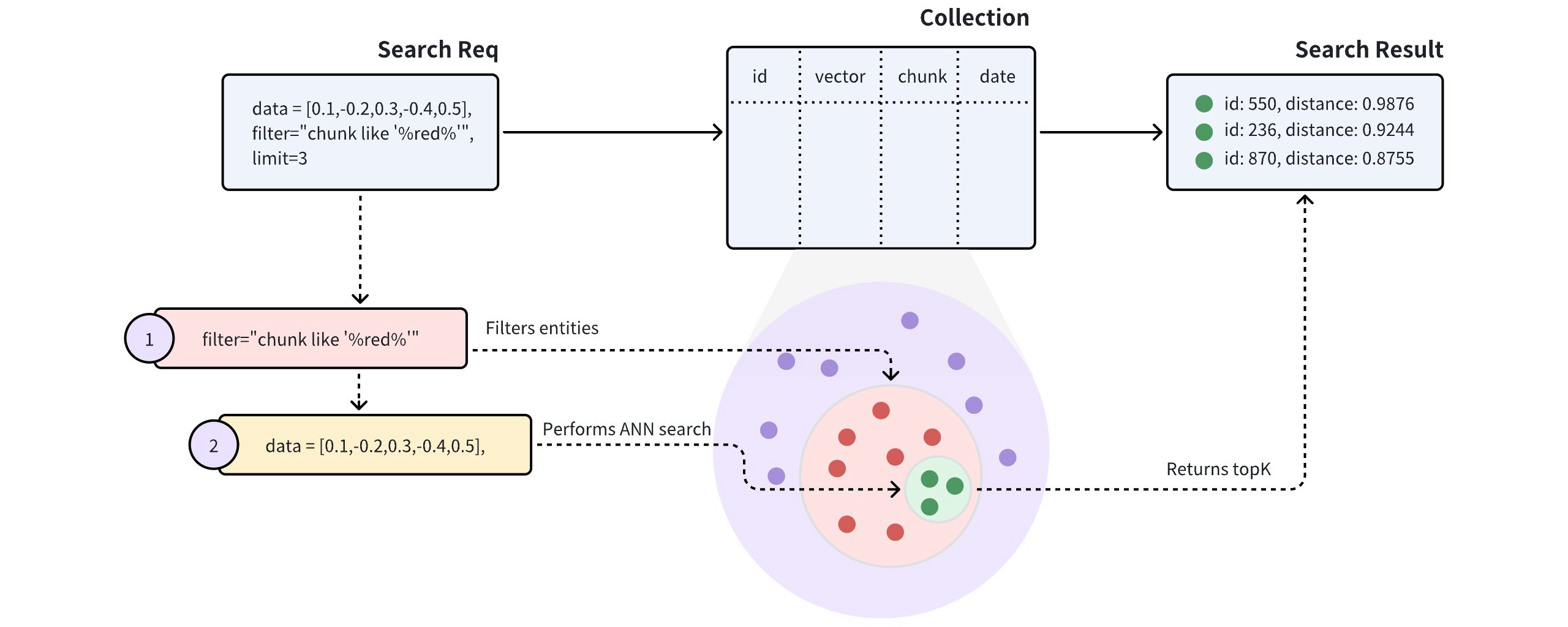
As shown in the above diagram, the search request carries chunk like "%red%" as the filtering condition, indicating that Milvus should conduct the ANN search within all the entities that have the word red in the chunk field. Specifically, Milvus does the following:
- Filtering entities that match the filtering conditions carried in the search request.
- Conduct the ANN search within the filtered entities.
- Returns top-K entities.
# Iterative filtering
The standard filtering process effectively narrows the search scope to a small range. However, overly complex filtering expressions may result in very high search latency. In such cases, iterative filtering can serve as an alternative, helping to reduce the workload of scalar filtering.
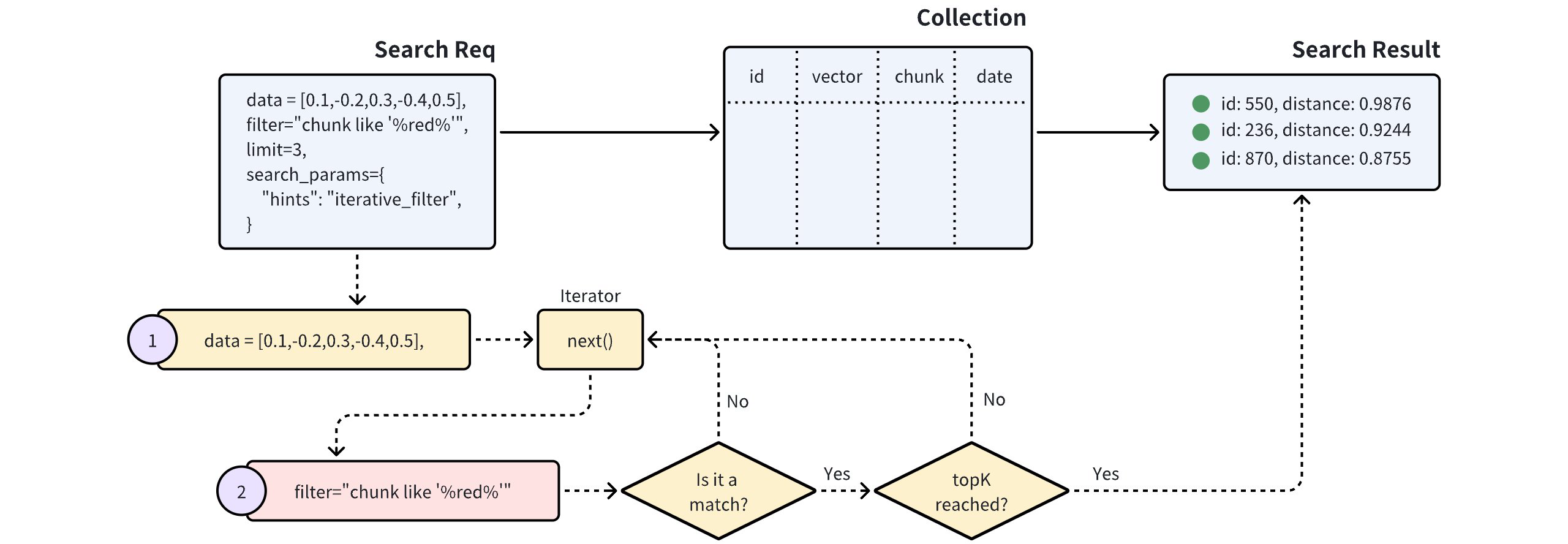
As illustrated in the diagram above, a search with iterative filtering performs the vector search in iterations. Each entity returned by the iterator undergoes scalar filtering, and this process continues until the specified topK results are achieved.
This method significantly reduces the number of entities subjected to scalar filtering, making it especially beneficial for handling highly complex filtering expressions.
However, it's important to note that the iterator processes entities one at a time. This sequential approach can lead to longer processing times or potential performance issues, especially when a large number of entities are subjected to scalar filtering.
# Examples
This section demonstrates how to conduct a filtered search. Code snippets in this section assume you already have the following entities in your collection. Each entity has four fields, namely id, vector, color, and likes.
[
{
"id": 0,
"vector": [
0.3580376395471989,
-0.6023495712049978,
0.18414012509913835,
-0.26286205330961354,
0.9029438446296592
],
"color": "pink_8682",
"likes": 165
},
{
"id": 1,
"vector": [
0.19886812562848388,
0.06023560599112088,
0.6976963061752597,
0.2614474506242501,
0.838729485096104
],
"color": "red_7025",
"likes": 25
},
{
"id": 2,
"vector": [
0.43742130801983836,
-0.5597502546264526,
0.6457887650909682,
0.7894058910881185,
0.20785793220625592
],
"color": "orange_6781",
"likes": 764
},
{
"id": 3,
"vector": [
0.3172005263489739,
0.9719044792798428,
-0.36981146090600725,
-0.4860894583077995,
0.95791889146345
],
"color": "pink_9298",
"likes": 234
},
{
"id": 4,
"vector": [
0.4452349528804562,
-0.8757026943054742,
0.8220779437047674,
0.46406290649483184,
0.30337481143159106
],
"color": "red_4794",
"likes": 122
},
{
"id": 5,
"vector": [
0.985825131989184,
-0.8144651566660419,
0.6299267002202009,
0.1206906911183383,
-0.1446277761879955
],
"color": "yellow_4222",
"likes": 12
},
{
"id": 6,
"vector": [
0.8371977790571115,
-0.015764369584852833,
-0.31062937026679327,
-0.562666951622192,
-0.8984947637863987
],
"color": "red_9392",
"likes": 58
},
{
"id": 7,
"vector": [
-0.33445148015177995,
-0.2567135004164067,
0.8987539745369246,
0.9402995886420709,
0.5378064918413052
],
"color": "grey_8510",
"likes": 775
},
{
"id": 8,
"vector": [
0.39524717779832685,
0.4000257286739164,
-0.5890507376891594,
-0.8650502298996872,
-0.6140360785406336
],
"color": "white_9381",
"likes": 876
},
{
"id": 9,
"vector": [
0.5718280481994695,
0.24070317428066512,
-0.3737913482606834,
-0.06726932177492717,
-0.6980531615588608
],
"color": "purple_4976",
"likes": 765
}
]
2
3
4
5
6
7
8
9
10
11
12
13
14
15
16
17
18
19
20
21
22
23
24
25
26
27
28
29
30
31
32
33
34
35
36
37
38
39
40
41
42
43
44
45
46
47
48
49
50
51
52
53
54
55
56
57
58
59
60
61
62
63
64
65
66
67
68
69
70
71
72
73
74
75
76
77
78
79
80
81
82
83
84
85
86
87
88
89
90
91
92
93
94
95
96
97
98
99
100
101
102
103
104
105
106
107
108
109
110
111
112
113
114
115
116
117
118
119
120
121
122
# Search with standard filtering
The following code snippets demonstrate a search with standard filtering, and the request in the following code snippet carries a filtering condition and several output fields.
from pymilvus import MilvusClient
client = MilvusClient(
uri="http://localhost:19530",
token="root:Milvus"
)
query_vector = [0.3580376395471989, -0.6023495712049978, 0.18414012509913835, -0.26286205330961354, 0.9029438446296592]
res = client.search(
collection_name="my_collection",
data=[query_vector],
limit=5,
filter='color like "red%" and likes > 50',
output_fields=["color", "likes"]
)
for hits in res:
print("TopK results:")
for hit in hits:
print(hit)
2
3
4
5
6
7
8
9
10
11
12
13
14
15
16
17
18
19
20
21
The filtering condition carried in the search request reads color like "red%" and likes > 50. It uses the and operator to include two conditions: the first one asks for entities that have a value starting with red in the color field, and the other asks for entities with a value greater than 50 in the likes field. There are only two entities meeting these requirements. With the top-K set to 3, Milvus will calculate the distance between these two entities to the query vector and return them as the search results.
[
{
"id": 4,
"distance": 0.3345786594834839,
"entity": {
"vector": [
0.4452349528804562,
-0.8757026943054742,
0.8220779437047674,
0.46406290649483184,
0.30337481143159106
],
"color": "red_4794",
"likes": 122
}
},
{
"id": 6,
"distance": 0.6638239834383389,
"entity": {
"vector": [
0.8371977790571115,
-0.015764369584852833,
-0.31062937026679327,
-0.562666951622192,
-0.8984947637863987
],
"color": "red_9392",
"likes": 58
}
}
]
2
3
4
5
6
7
8
9
10
11
12
13
14
15
16
17
18
19
20
21
22
23
24
25
26
27
28
29
30
31
32
For more information on the operators you can use in metadata filtering, refer to Filtering.
# Search iterative filtering
To conduct a filtered search with iterative filtering, you can do as follow:
from pymilvus import MilvusClient
client = MilvusClient(
uri="http://localhost:19530",
token="root:Milvus"
)
query_vector = [0.3580376395471989, -0.6023495712049978, 0.18414012509913835, -0.26286205330961354, 0.9029438446296592]
res = client.search(
collection_name="my_collection",
data=[query_vector],
limit=5,
filter='color like "red%" and likes > 50',
output_fields=["color", "likes"],
search_params={
"hints": "iterative_filter"
}
)
for hits in res:
print("TopK results:")
for hit in hits:
print(hit)
2
3
4
5
6
7
8
9
10
11
12
13
14
15
16
17
18
19
20
21
22
23
24
# Range Search
A range search improves search result relevancy by restricting the distance or score of the returned entities within a specific range. This page helps you understand what range search is and the procedures to conduct a range search.
# Overview
When executing a Range Search request, Milvus uses the most similar vectors to the query vector from the ANN Search results as the center, with the radius specified in the Search request as the outer circle's radius, and the range_filter as the inner circle's radius to draw two concentric cicles. All vectors with similarity scores that fall within the anular region formed by these two concentric circles will be returned. Here, the range_filter can be set to 0, indicating that all entities within the specified similarity score (radius) will be returned.
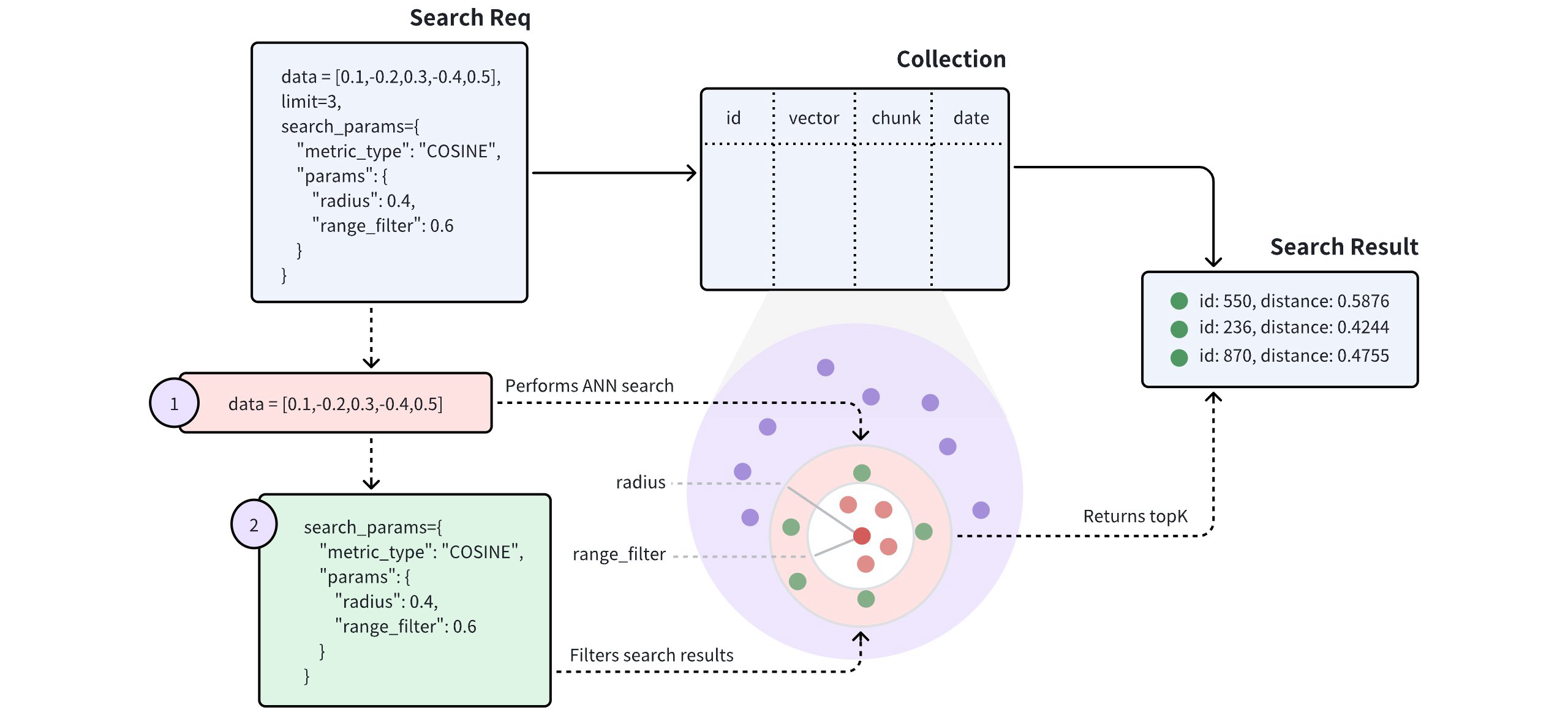
The above diagram shows that a range search request carries two parameters: radius and range_filter. Upon receiving a range search request, Milvus does the following:
- Use the specified metric type (COSINE) to find all vector embeddings most similar to the query vector.
- Filter the vector embeddings whose distance or scores to the query vector fall within the range specified by the radius and range_filter parameters.
- Return the top-K entities from the filtered ones.
The way to set radius and range_filter varies with the metric type of the search. The following table lists the requirements for setting these two parameters with different metric types.
| Metric Type | Denotations | Requirements for Setting radius and range_filter |
|---|---|---|
L2 | A smaller L2 distance indicates a higher similarity | To ignore the most similar vector embeddings, ensure that range_filter <= distance < radius |
IP | A greater IP distance indicates a higher similarity | To ignore the most similar vector embeddings, ensure that radius < distance <= range_filter |
COSINE | A greater COSINE distance indicates a higher similarity. | To ignore the most similar vector embeddings, ensure that radius < distance <= range_filter |
JACCARD | A smaller Jaccard distance indicates a higher similarity | To ingore the most similar vector embeddings, ensure that range_filter <= distance < radius |
HAMMING | A smaller Hamming distance indicates a higher similarity. | To ignore the most similar vector embeddings, ensure that range_filter <= distance < radius |
# Examples
This section demonstrates how to conduct a range search. The search requests in the following code snippets do not carry a metric type, indicating the default metric type COSINE applies. In this case, ensure that the radius value is smaller than the range_filter value.
In the following code snippets, set radius to 0.4 and range_filter to 0.6 so that Milvus returns all entities whose distances or scores to the query vector fall within 0.4 to 0.6.
from pymilvus import MilvusClient
client = MilvusClient(
uri="http://localhost:19530",
token="root:Milvus"
)
query_vector = [0.3580376395471989, -0.6023495712049978, 0.18414012509913835, -0.26286205330961354, 0.9029438446296592]
res = client.search(
collection_name="my_collection",
data=[query_vector],
limit=3,
search_params={
# highlight-start
"params": {
"radius": 0.4,
"range_filter": 0.6
}
# highlight-end
}
)
for hits in res:
print("TopK results:")
for hit in hits:
print(hit)
2
3
4
5
6
7
8
9
10
11
12
13
14
15
16
17
18
19
20
21
22
23
24
25
26
27
# Grouping Search
A grouping search allows Milvus to group the search results by the values in a specified field to aggregate data at a higher level. For example, you can use a basic ANN search to find books similar to the one at hand, but you can use a grouping search to find the book categories that may involve the topics discussed in that book. This topic describes how to use Grouping Search along with key considerations.
# Overview
When entities in the search results share the same value in a scalar field, this indicates that they are similar in a particular attribute, which may negatively impact the search results.
Assume a collection stores multiple documents (denoted by docId). To retain as much semantic information as possible when coverting documents into vectors, each document is split into smaller, manageable paragraphs (or chunks) and stored as separate entities. Even though the document is divided into smaller sections, users are often still interested in identifying which documents are most relevant to their needs.
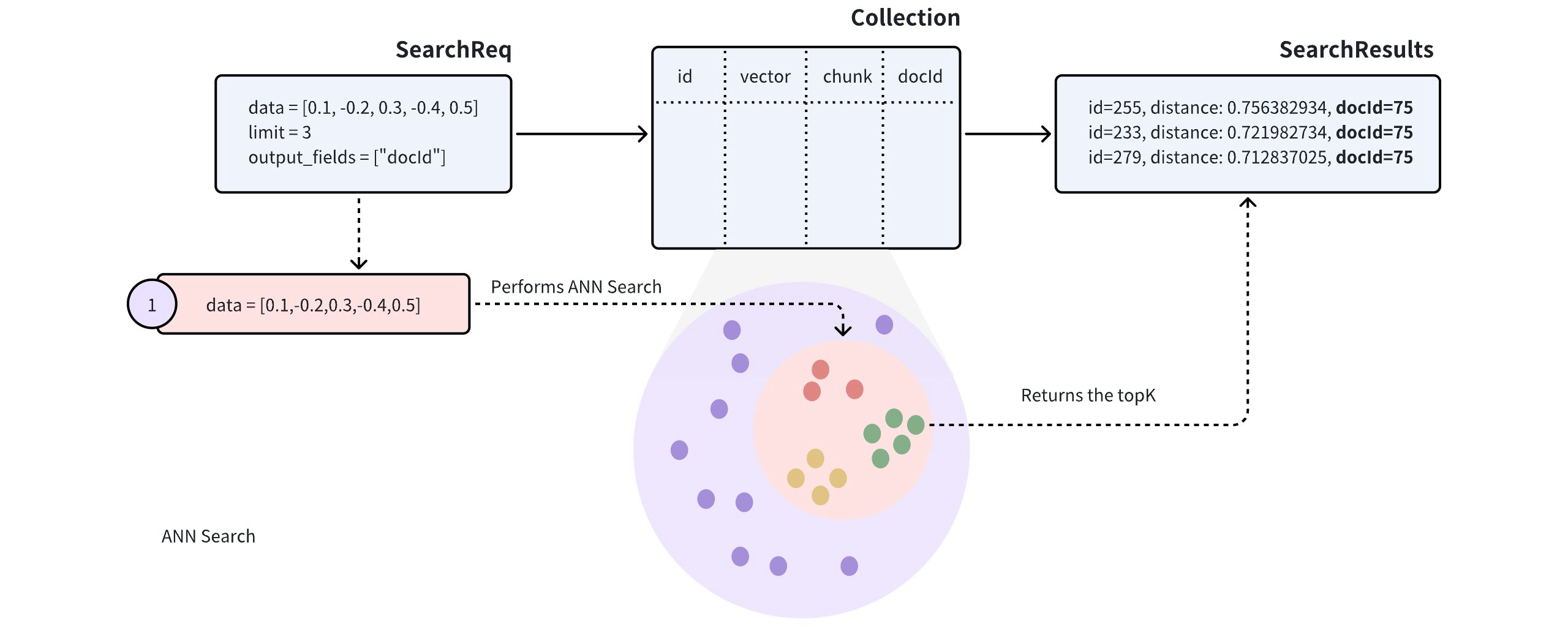
When performing an Approximate Nearest Neighbor (ANN) search on such a collection, the search results may include several paragraphs from the same document, potentially causing other documents to be overlooked, which may not align with the intended use case.
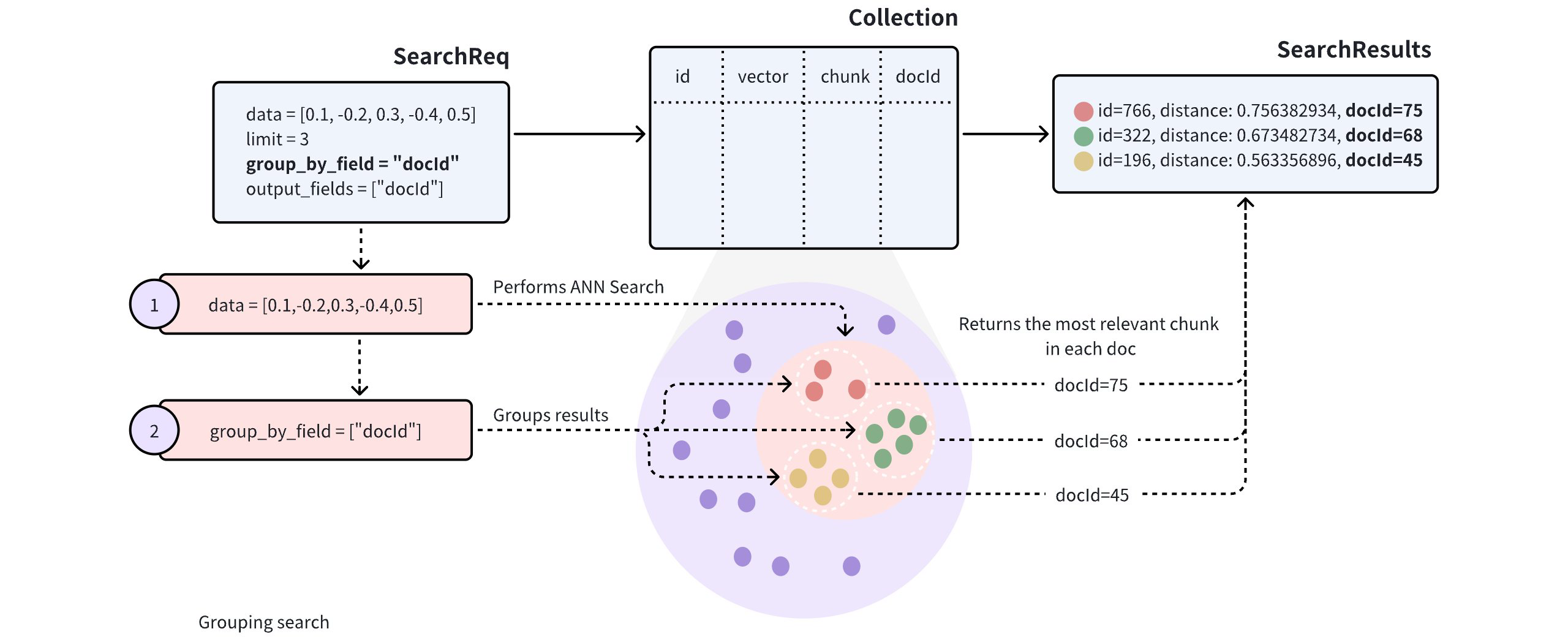
To improve the diversity of search results, you can add the group_by_field parameter in the search request to enable Grouping Search. As shown in the diagram, you can set group_by_field to docId. Upon receiving this request, Milvus will:
- Perform an ANN search based on the provided query vector to find all entities most similar to the query.
- Group the search results by the specified
group_by_field, such asdocId. - Return the top results for each group, as defined by the
limitparameter, with the most similar entity from each group.
NOTE
By default, Grouping Search returns only one entity per group. If you want to increase the number of results to return per group, you can control this with the group_size and strict_group_size parameters.
# Perform Grouping Search
This section provides example code to demonstrate the use of Grouping Search. The following example assumes the collection includes fields for id, vector, chunk, and docId.
[
{
"id": 0,
"vector": [
0.3580376395471989,
-0.6023495712049978,
0.18414012509913835,
-0.26286205330961354,
0.9029438446296592
],
"chunk": "pink_8682",
"docId": 1
},
{
"id": 1,
"vector": [
0.19886812562848388,
0.06023560599112088,
0.6976963061752597,
0.2614474506242501,
0.838729485096104
],
"chunk": "red_7025",
"docId": 5
},
{
"id": 2,
"vector": [
0.43742130801983836,
-0.5597502546264526,
0.6457887650909682,
0.7894058910881185,
0.20785793220625592
],
"chunk": "orange_6781",
"docId": 2
},
{
"id": 3,
"vector": [
0.3172005263489739,
0.9719044792798428,
-0.36981146090600725,
-0.4860894583077995,
0.95791889146345
],
"chunk": "pink_9298",
"docId": 3
},
{
"id": 4,
"vector": [
0.4452349528804562,
-0.8757026943054742,
0.8220779437047674,
0.46406290649483184,
0.30337481143159106
],
"chunk": "red_4794",
"docId": 3
},
{
"id": 5,
"vector": [
0.985825131989184,
-0.8144651566660419,
0.6299267002202009,
0.1206906911183383,
-0.1446277761879955
],
"chunk": "yellow_4222",
"docId": 4
},
{
"id": 6,
"vector": [
0.8371977790571115,
-0.015764369584852833,
-0.31062937026679327,
-0.562666951622192,
-0.8984947637863987
],
"chunk": "red_9392",
"docId": 1
},
{
"id": 7,
"vector": [
-0.33445148015177995,
-0.2567135004164067,
0.8987539745369246,
0.9402995886420709,
0.5378064918413052
],
"chunk": "grey_8510",
"docId": 2
},
{
"id": 8,
"vector": [
0.39524717779832685,
0.4000257286739164,
-0.5890507376891594,
-0.8650502298996872,
-0.6140360785406336
],
"chunk": "white_9381",
"docId": 5
},
{
"id": 9,
"vector": [
0.5718280481994695,
0.24070317428066512,
-0.3737913482606834,
-0.06726932177492717,
-0.6980531615588608
],
"chunk": "purple_4976",
"docId": 3
}
]
2
3
4
5
6
7
8
9
10
11
12
13
14
15
16
17
18
19
20
21
22
23
24
25
26
27
28
29
30
31
32
33
34
35
36
37
38
39
40
41
42
43
44
45
46
47
48
49
50
51
52
53
54
55
56
57
58
59
60
61
62
63
64
65
66
67
68
69
70
71
72
73
74
75
76
77
78
79
80
81
82
83
84
85
86
87
88
89
90
91
92
93
94
95
96
97
98
99
100
101
102
103
104
105
106
107
108
109
110
111
112
113
114
115
116
117
118
119
120
121
122
In the search request, set both group_by_field and output_fields to docId. Milvus will group the results by the specified field and return the most similar entity from each group, including the value of docId for each returned entity.
from pymilvus import MilvusClient
client = MilvusClient(
uri="http://localhost:19530",
token="root:Milvus"
)
query_vectors = [[0.14529211512077012, 0.9147257273453546, 0.7965055218724449, 0.7009258593102812, 0.5605206522382088]]
# Group search results
res = client.search(
collection_name="my_collection",
data=query_vectors,
limit=3,
group_by_field="docId",
output_fields=["docId"]
)
# Retrieve the values in the docId column
doc_ids = [result['entity']['docId'] for result in res[0]]
2
3
4
5
6
7
8
9
10
11
12
13
14
15
16
17
18
19
20
In the request above, limit=3 indicates that the system will return search results from three groups, with each group containing the single most similar entity to the query vector.
# Configure group size
By default, Grouping Search returns only one entity per group. If you want multiple results per group, adjust the group_size and strict_group_size parameters.
# Group search results
res = client.search(
collection_name="my_collection" ,
data=query_vectors, # query vector
limit=5, # Number of groups to return
group_by_field="docId", # grouping field
group_size=2, # p to 2 entities to return from each group
strict_group_size=True, # return exact 2 entities from each group
output_fields=["docId"]
)
2
3
4
5
6
7
8
9
10
In the example above:
group_size: Specifies the desired number of entities to return per group. For instance, settinggroup_size=2means each group (or eachdocId) should ideally return two of the most similar paragraphs (or chunks). Ifgroup_sizeis not set, the system defaults to returning one result per group.strict_group_size: This boolean parameter controls whether the system should strictly enforce the count set bygroup_size. Whenstrict_group_size=True, the system will attempt to include the exact number of entities specified bygroup_sizein each group (e.g., two paragraphs), unless there isn't enough data in that group. By default (strict_group_size=False), the system prioritizes metting the number of groups specified by thelimitparameter, rather than ensuring each group containsgroup_sizeentities. This approach is generally more efficient in cases where data distribution is uneven.
For additional parameter details, refer to Search.
# Considerations
- Indexing: This grouping feature works only for collections that are indexed with these index types: FLAT, IVF_FLAT, IVF_SQ8, HNSW, HNSW_PQ, HNSW_PRQ, HNSW_SQ, DISKANN, SPARSE_INVERTED_INDEX.
- Number of groups: The
limitparameter controls the number of groups from which search results are returned, rather than the specific number of entities within each group. Setting an appropriatelimithelps control search diversity and query performance. Reducinglimitcan reduce computation costs if data is densely distributed or performance is a concern. - Entities per group: The
group_sizeparameter controls the number of entities returned per group. Adjustinggroup_sizebased on your use can increase the richness of search results. However, if data is unevenly distributed, some groups may return fewer entities than specified bygroup_size, particularly in limited data scenarios. - Strict group size: When
strict_group_size=True, the system will attempt to return the specified number of entities (group_size) for each group, unless there isn't enough data in that group. This setting ensures consistent entity counts per group but may lead to performance degradation with uneven data distribution or limited resources. If strict entity counts aren't required, settingstrict_group_size=Falsecan improve query speed.
# Hybrid Search
In many applications, an object can be searched by a rich set of information such as title an description, or with multiple modalities such as text, images, and audio. For example, a tweet with a piece of text and an image shall be searched if either the text or the image matches the semantic of the search query. Hybrid search enhances search experience by combining searches across these diverse fields. Milvus supports this by allowing search on multiple vector fields, conducting several Approximate Nearest Neighbor (ANN) searches simultaneously. Multi-vector hybrid search is particularly useful if you want to search both text and images, multiple text fields that describe the same object, or dense and sparse vectors to improve search quality.
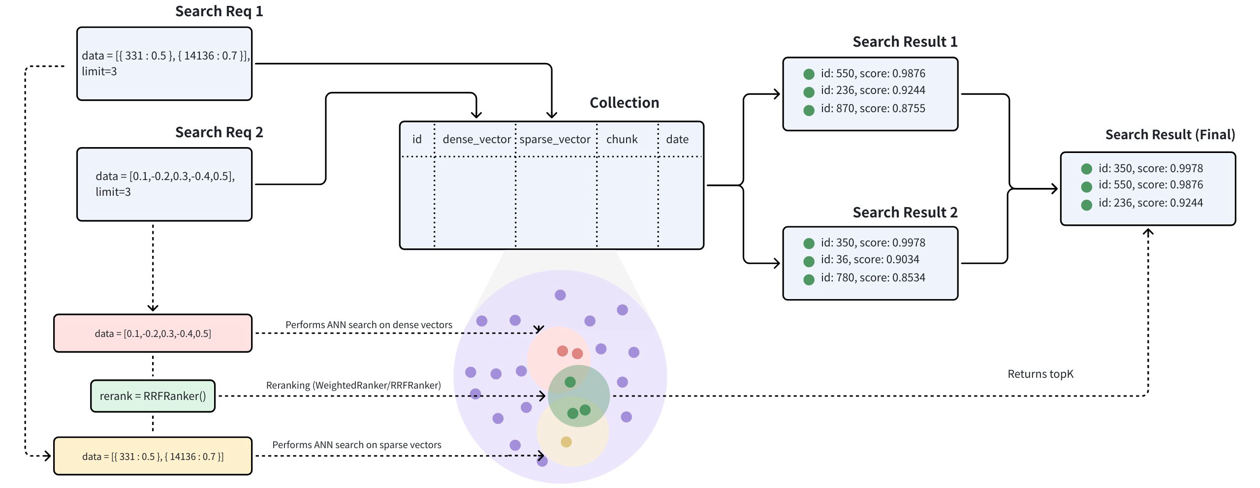
The multi-vector hybrid search integrates different search methods or spans embeddings from various modalities:
- Sparse-Dense Vector Search: Dense Vector are excellent for capturing semantic relationships, while Sparse Vector are highly effective for precise keyword matching. Hybrid search combines these approaches to provide both a broad conceptual understanding and exact term relevance, thus improving search results. By leveraging the strengths of each method, hybrid search overcomes the limitations of indiviual approaches, offering better performance for complex queries. Here is more detailed guide on hybrid retrieval that combines sementic search with full-text search.
- Multimodal Vector Search: Multimodal vector search is a powerful technique that allows you to search across various data types, including text, images, audio, and others. The main advantage of this approach is its ability to unify different modalities into a seamless and cohesive search experience. For instance, in product search, a user might input a text query to find products described with both text and images. By combining these modalities through a hybrid search method, you can enhance search accuracy or enrich the search results.
# Example
Let's consider a real world use case where each product includes a text description and an image. Based on the available data, we can conduct three types of searches:
- Semenatic Text Search: This involves querying the text description of the product using dense vectors. Text embeddings can be generated using models such as BERT and Transformers or services like OpenAI.
- Full-Text Search: Here, we query the text description of the product using a keyword match with sparse vectors. Algorithms like BM25 or sparse embedding modesl such as BGE-M3 or SPLADE can be utilized for this purpose.
- Multimodal Image Search: This method queries over the image using a text query with dense vectors. Image embeddings can be generated with models like CLIP.
This guide will walk you through an example of a multimodal hybrid search combining the above search methods, given the raw text description and image embeddings of products. We will demonstrate how to store multi-vector data and perform hybrid searches with a reranking strategy.
# Create a collection with multiple vector fields
The process of creating a collection involves three key steps: defining the collection schema, configuring the index parameters, and creating the collection.
# Define schema
For multi-vector hybrid search, we should define multiple vector fields within a collection schema. For details about the limits on the number of vector fields allowed in a collection, see Zilliz Cloud Limits. However, if necessary, you can adjust the proxy.maxVectorFieldNum to include up to 10 vector fields in a collection as needed.
This example incorporates the following fields into the schema:
id: Serves as the primary key for storing text IDs. This field is of data typeINT64.text: Used for storing textual content. This field is of the data typeVARCHARwith a maximum length of 1000 bytes. Theenable_analyzeroption is set toTrueto facilitate full-text search.text_dense: Used to store dense vectors of the texts. This field is of the data typeFLOAT_VECTORwith a vector dimension of 768.text_sparse: Used to store sparse vectors of the texts. This field is of the data typeSPARSE_FLOAT_VECTOR.image_dense: Used to store dense vectors of the product images. This field is of the data typeFLOAT_VECTORwith a vector dimension of 512.
Since we will use the built-in BM25 algorithm to perform a full-text search on the text field, it is necessary to add the Milvus Function to the schema. For further details, please refer to Full Text Search.
from pymilvus import (
MilvusClient, DataType, Function, FunctionType
)
client = MilvusClient(
uri="http://localhost:19530",
token="root:Milvus"
)
# Init schema with auto_id disabled
schema = client.create_schema(auto_id=False)
# Add fields to schema
schema.add_field(field_name="id", datatype=DataType.INT64, is_primary=True, description="product id")
schema.add_field(
field_name="text",
datatype=DataType.VARCHAR,
max_length=1000,
enable_analyzer=True,
description="raw text of product description")
schema.add_field(
field_name="text_dense",
datatype=DataType.FLOAT_VECTOR,
dim=768,
description="text dense embedding"
)
schema.add_field(
field_name="text_sparse",
datatype=DataType.SPARSE_FLOAT_VECTOR,
description="text sparse embedding auto-generated by the built-in BM25 function"
)
schema.add_field(
field_name="image_dense",
datatype=DataType.FLOAT_VECTOR,
dim=512,
description="image dense embedding"
)
# Add function to schema
bm25_function = Function(
name="text_bm25_emb",
input_field_names=["text"],
output_field_names=["text_sparse"],
function_type=FunctionType.BM25
)
schema.add_function(bm25_function)
2
3
4
5
6
7
8
9
10
11
12
13
14
15
16
17
18
19
20
21
22
23
24
25
26
27
28
29
30
31
32
33
34
35
36
37
38
39
40
41
42
43
44
45
46
# Create index
After defining the collection schema, the next step is to configure the vector indexes and specify the similarity metrics. In the given example:
text_dense_index: an index of typeAUTOINDEXwithIPmetric type is created for the text dense vector field.text_sparse_index: an index of typeSPARSE_INVERTED_INDEXwithBM25metric type is used for the text sparse vector field.image_dense_index: an index of typeAUTOINDEXwithIPmetric type is created for the image dense vector field.
You can choose other index types as necessary to best suit your needs and data types. For further information on the supported index types, please refer to the documentation on available index types.
index_params = client.prepare_index_params()
index_params.add_index(
field_name="text_dense",
index_name="text_dense_index",
index_type="AUTOINDEX",
metric_type="IP"
)
index_params.add_index(
field_name="text_sparse",
index_name="text_sparse_index",
index_type="SPARSE_INVERTED_INDEX",
metric_type="BM25",
params={"inverted_index_algo": "DAAT_MAXSCORE"}, # or "DAAT_WAND" or "TAAT_NAIVE"
)
index_params.add_index(
field_name="image_dense",
index_name="image_dense_index",
index_type="AUTOINDEX",
metric_type="IP"
)
2
3
4
5
6
7
8
9
10
11
12
13
14
15
16
17
18
19
20
21
22
23
# Create collection
Create a collection named demo with the collection schema and indexes configured in the previous two steps.
client.create_collection(
collection_name="my_collection",
schema=schema,
index_params=index_params
)
2
3
4
5
# Insert data
This section inserts data into the my_collection collection based on the schema defined earlier. During insert, ensure all field, except those with auto-generated values, are provided with data in the correct format. In this example:
id: an integer representing the product IDtext: a string containing the product descriptiontext_dense: a list of 768 floating-point values representing the dense embedding of the text descriptionimage_dense: a list of 512 floating-point values representing the dense embedding of the product image.
You may use the same or different models to generate dense embeddings for each field. In this example, the two dense embeddings have different dimensions, suggesting they were generated by different models. When defining each search later, be sure to use the corresponding model to generate the appropriate query embedding.
Since this example uses the built-in BM25 function to generate sparse embeddings from the text field, you do not need to supply sparse vectors manually. However, if you opt not to use BM25, you must precompute and provide the sparse embeddings yourself.
import random
def generate_dense_vector(dim):
return [random.random() for _ in range(dim)]
data=[
{
"id": 0,
"text": "Red cotton t-shirt with round neck",
"text_dense": generate_dense_vector(768),
"image_dense": generate_dense_vector(512)
},
{
"id": 1,
"text": "Wireless noise-cancelling over-ear headphones",
"text_dense": generate_dense_vector(768),
"image_dense": generate_dense_vector(512)
},
{
"id": 2,
"text": "Stainless steel water bottle, 500ml",
"text_dense": generate_dense_vector(768),
"image_dense": generate_dense_vector(512)
}
]
res = client.insert(
collection_name="my_collection",
data=data
)
2
3
4
5
6
7
8
9
10
11
12
13
14
15
16
17
18
19
20
21
22
23
24
25
26
27
28
29
30
# Perform Hybrid Search
# Step 1: Create multiple AnnSearchRequest instances
Hybrid Search is implemented by creating multiple AnnSearchRequest in the hybrid_search() function, where each AnnSearchRequest represents a basic ANN search request for a specific vector field. Therefore, before conducting a Hybrid Search, it is necessary to create an AnnSearchRequest for each vector field.
In addition, by configuring the expr parameter in an AnnSearchRequest, you can set the filtering conditions for your hybrid search. Please refer to Filtered Search and Filtering Explained.
NOTE
In Hybrid Search, each AnnSearchRequest supports only one query data.
To demonstrate the capabilities of various search vector fields, we will construct three AnnSearchRequest search requests using a sample query. We will also use its pre-computed dense vectors for this process. The search requests will target the following vector fields:
text_densefor semantic text search, allowing for contextual understanding and retrieval based on meaning rather than direct keyword matching.text_sparsefor full-text search for keyword matching, focusing on exact word or phrase matches within the text.image_densefor multimodal text-to-image search, to retrieve relevant product images based on the semantic content of the query.
from pymilvus import AnnSearchRequest
query_text = "white headphones, quiet and comfortable"
query_dense_vector = generate_dense_vector(768)
query_multimodal_vector = generate_dense_vector(512)
# text semantic search (dense)
search_param_1 = {
"data": [query_dense_vector],
"anns_field": "text_dense",
"param": {"nprobe": 10},
"limit": 2
}
request_1 = AnnSearchRequest(**search_param_1)
# full-text search (sparse)
search_param_2 = {
"data": [query_text],
"anns_field": "text_sparse",
"param": {"drop_ratio_search": 0.2},
"limit": 2
}
request_2 = AnnSearchRequest(**search_param_2)
# text-to-image search (multimodal)
search_param_3 = {
"data": [query_multimodal_vector],
"anns_field": "image_dense",
"param": {"nprobe": 10},
"limit": 2
}
request_3 = AnnSearchRequest(**search_param_3)
reqs = [request_1, request_2, request_3]
2
3
4
5
6
7
8
9
10
11
12
13
14
15
16
17
18
19
20
21
22
23
24
25
26
27
28
29
30
31
32
33
34
Given that the parameter limit is set to 2, each AnnSearchRequest returns 2 search results. In this example, 3 AnnSearchRequest instances are created, resulting in a total of 6 search results.
# Step 2: Configure a reranking strategy
To merge and rerank the sets of ANN search results, selecting an appropriate reranking strategy is essential. Milvus offers several types of reranking strategies. For more details on these reranking mechanisms, please refer to Weighted Ranker or RRF Ranker.
In this example, since there is no particular emphasis on specific search queries, we will proceed with the RRFRanker strategy.
ranker = Function(
name="rrf",
input_field_names=[], # Must be an empty list
function_type=FunctionType.RERANK,
params={
"reranker": "rrf",
"k": 100 # Optional
}
)
2
3
4
5
6
7
8
9
# Step 3: Perform a Hybrid Search
Before initiating a Hybrid Search, ensure that the collection is loaded. If any vector fields within the collection lack an index or are not loaded into memory, an error will occur upon executing the Hybrid Search method.
res = client.hybrid_search(
collection_name="my_collection",
reqs=reqs,
ranker=ranker,
limit=2
)
for hits in res:
print("TopK results:")
for hit in hits:
print(hit)
2
3
4
5
6
7
8
9
10
The following is the output:
["['id: 1, distance: 0.006047376897186041, entity: {}', 'id: 2, distance: 0.006422005593776703, entity: {}']"]
With the limit=2 parameter specified for the Hybrid Search, Milvus will rerank the six results obtained from the three searches. Ultimately, they will return only the top two most similar results.
# Query
In addition to ANN searches, Milvus also supports metadata filtering through queries. This page introduces how to use Query, Get, and QueryIterators to perform metadata filtering.
NOTE
If you dynamically add new fields after the collection has been created, queries that include these fields will return the defined default values or NULL for entities that have not explicitly set values. For details, refer to Add Fields to an Existing Collection.
# Overview
A collection can store various types of scalar fields. You can have Milvus filter Entities based on one or more scalar fields. Milvus offers three types of queries: Query, Get, and QueryIterator. The table below compares these three query types.
| Type | Get | Query | QueryIterator |
|---|---|---|---|
| Applicable scenarios | To find entities that hold the specified primary keys. | To find all or a specified number of entities that meet the custom filtering conditions. | To find all entities that meet the custom filtering conditions in paginated queries. |
| Filtering method | By Primary keys | by filtering expressions | By filtering expressions. |
| Mandatory parameters | 1. Collection name 2. Primary keys | 1. Collection name 2. Filtering expressions | 1. Colection name 2. Filtering expressions 3. Number of entities to return per query |
| Optional parameters | 1. Partition name 2. Output fields | 1. Partition Name 2. Number of entities to return 3. Output fields | 1. Partition name 2. Number of entities to return in total 3. Output fields |
| Returns | Returns entities that hold the specified primary keys in the specified collection or partition. | Returns all or a specified number of entities that meet the custom filtering conditions in the specified collection or partition. | Returns all entities that meet the custom filtering conditions in the specified collection or partition through paginated queries. |
# Use Get
when you need to find entities by their primary keys, you can use the Get method. The following code examples assume that there are three fields named id, vector, and color in your collection.
[
{
"id": 0,
"vector": [
0.3580376395471989,
-0.6023495712049978,
0.18414012509913835,
-0.26286205330961354,
0.9029438446296592
],
"color": "pink_8682"
},
{
"id": 1,
"vector": [
0.19886812562848388,
0.06023560599112088,
0.6976963061752597,
0.2614474506242501,
0.838729485096104
],
"color": "red_7025"
},
{
"id": 2,
"vector": [
0.43742130801983836,
-0.5597502546264526,
0.6457887650909682,
0.7894058910881185,
0.20785793220625592
],
"color": "orange_6781"
},
{
"id": 3,
"vector": [
0.3172005263489739,
0.9719044792798428,
-0.36981146090600725,
-0.4860894583077995,
0.95791889146345
],
"color": "pink_9298"
},
{
"id": 4,
"vector": [
0.4452349528804562,
-0.8757026943054742,
0.8220779437047674,
0.46406290649483184,
0.30337481143159106
],
"color": "red_4794"
},
{
"id": 5,
"vector": [
0.985825131989184,
-0.8144651566660419,
0.6299267002202009,
0.1206906911183383,
-0.1446277761879955
],
"color": "yellow_4222"
},
{
"id": 6,
"vector": [
0.8371977790571115,
-0.015764369584852833,
-0.31062937026679327,
-0.562666951622192,
-0.8984947637863987
],
"color": "red_9392"
},
{
"id": 7,
"vector": [
-0.33445148015177995,
-0.2567135004164067,
0.8987539745369246,
0.9402995886420709,
0.5378064918413052
],
"color": "grey_8510"
},
{
"id": 8,
"vector": [
0.39524717779832685,
0.4000257286739164,
-0.5890507376891594,
-0.8650502298996872,
-0.6140360785406336
],
"color": "white_9381"
},
{
"id": 9,
"vector": [
0.5718280481994695,
0.24070317428066512,
-0.3737913482606834,
-0.06726932177492717,
-0.6980531615588608
],
"color": "purple_4976"
}
]
2
3
4
5
6
7
8
9
10
11
12
13
14
15
16
17
18
19
20
21
22
23
24
25
26
27
28
29
30
31
32
33
34
35
36
37
38
39
40
41
42
43
44
45
46
47
48
49
50
51
52
53
54
55
56
57
58
59
60
61
62
63
64
65
66
67
68
69
70
71
72
73
74
75
76
77
78
79
80
81
82
83
84
85
86
87
88
89
90
91
92
93
94
95
96
97
98
99
100
101
102
103
104
105
106
107
108
109
110
111
112
You can get entities by their IDs as follow.
from pymilvus import MilvusClient
client = MilvusClient(
uri="http://localhost:19530",
token="root:Milvus"
)
res = client.get(
collection_name="my_collection",
ids=[0, 1, 2],
output_fields=["vector", "color"]
)
print(res)
2
3
4
5
6
7
8
9
10
11
12
13
14
# Use Query
When you need to find entities by custom filtering conditions, use the Query method. The following code examples assumes there are three fields named id, vector, and color and return the specified number of entities that hold a color value starting with red.
from pymilvus import MilvusClient
client = MilvusClient(
uri="http://localhost:19530",
token="root:Milvus"
)
res = client.query(
collection_name="my_collection",
filter="color like \"red%\",
output_fields=["vector", "color"],
limit=3
)
2
3
4
5
6
7
8
9
10
11
12
13
# Use QueryIterator
When you need to find entities by custom filtering conditions through paginated queries, create a QueryIterator and use its next() method to iterate over all entities to find those meeting the filtering conditions. The following code examples assume that there are three fields named id, vector, and color and return all entities that hold a color value starting with red.
from pymilvus import connections, Collection
connections.connect(
uri="http://localhost:19530",
token="root:Milvus"
)
collection = Collection("my_collection")
iterator = collection.query_iterator(
batch_size=10,
expr="color like \"red%\"",
output_fields=["color"]
)
results = []
while True:
result = iterator.next()
if not result:
iterator.close()
break
print(result)
results += result
2
3
4
5
6
7
8
9
10
11
12
13
14
15
16
17
18
19
20
21
22
23
24
25
# Queries in Partitions
You can also perform queries within one or multiple partitions by including the partition names in the Get, Query, or QueryIterator request. The following code examples assume that there is a partition named PartitionA in the collection.
from pymilvus import MilvusClient
client = MilvusClient(
uri="http://localhost:19530",
token="root:Milvus"
)
res = client.get(
collection_name="my_collection",
# highlight-next-line
partitionNames=["partitionA"],
ids=[10, 11, 12],
output_fields=["vector", "color"]
)
from pymilvus import MilvusClient
client = MilvusClient(
uri="http://localhost:19530",
token="root:Milvus"
)
res = client.query(
collection_name="my_collection",
# highlight-next-line
partitionNames=["partitionA"],
filter="color like \"red%\"",
output_fields=["vector", "color"],
limit=3
)
from pymilvus import connections, Collection
connections.connect(
uri="http://localhost:19530",
token="root:Milvus"
)
collection = Collection("my_collection")
iterator = collection.query_iterator(
# highlight-next-line
partition_names=["partitionA"],
batch_size=10,
expr="color like \"red%\"",
output_fields=["color"]
)
results = []
while True:
result = iterator.next()
if not result:
iterator.close()
break
print(result)
results += result
2
3
4
5
6
7
8
9
10
11
12
13
14
15
16
17
18
19
20
21
22
23
24
25
26
27
28
29
30
31
32
33
34
35
36
37
38
39
40
41
42
43
44
45
46
47
48
49
50
51
52
53
54
55
56
57
# Random Sampling with Query
To extract a representative subset of data from your collection for data exploration or development testing, use the RANDOM_SAMPLE(sampling_factor) expression, where the sampling_factor is a float between 0 and 1 representing the percentage of data to sample.
NOTE
For detailed usage, advanced examples, and best practices, refer to Random Sampling.
from pymilvus import MilvusClient
client = MilvusClient(
uri="http://localhost:19530",
token="root:Milvus"
)
res = client.query(
collection_name="my_collection",
# highlight-next-line
filter="RANDOM_SAMPLE(0.01)",
output_fields=["vector", "color"]
)
print(f"Sampled {len(res)} entities from collection")
res = client.query(
collection_name="my_collection",
# highlight-next-line
filter="color like \"red%\" AND RANDOM_SAMPLE(0.005)",
output_fields=["vector", "color"],
limit=10
)
print(f"Found {len(res)} red items in sample")
2
3
4
5
6
7
8
9
10
11
12
13
14
15
16
17
18
19
20
21
22
23
24
25
# Filtering
# Filtering Explained
Milvus provides powerful filtering capabilities that enable precise querying of your data. Filter expressions allow you to target specific scalar fields and refine search results with different conditions. This guide explains how to use filter expressions in Milvus, with examples focused on query operations. You can also apply these filters in search and delete requests.
# Basic operators
Milvus supports serveral basic operators for filtering data:
- Comparison Operators:
==,!=,>,<,>=, and<=allow filtering based on numeric or text fields. - Range Filters:
INandLIKEhelp match specific value ranges or sets. - Arithmetic Operators:
+,-,*,/,%, and**are used for calculations involving numeric fields. - Logical Operators:
AND,OR, andNOTcombine multiple conditions into complex expressions. - IS NULL and IS NOT NULL Operators: The
IS NULLandIS NOT NULLoperators are used to filter fields based on whether they contain a null value (absence of data), For details, refer to Basic Operators.
# Example: Filtering by Color
To find entities with primary colors (red, green, or blue) in a scalar field color, use the following filter expression:
filter='color in ["red", "green", "blue"]'
# Example: Filtering JSON Fields
Milvus allows referencing keys in JSON fields. For instance, if you have a JSON field product with keys price and model, and want to find products with a specific model and price lower than 1850, use this filter expression:
filter='product["model"] == "JSN-087" AND product["price"] < 1850'
# Example: Filtering Array Fields
If you have an array field history_temperatures containing the records of average temperatures reported by abservatories since the year 2000, and want to find observatories where the temperature in 2009 (the 10th recorded) exceeds 23℃, use this expression:
filter='history_temperatures[10] > 23'
For more information on these basic operators, refer to Basic Operators.
# Filter expression templates
When filtering using CJK characters, processing can be more complex due to their larger charater sets and encoding differences. This can result in slower performance, especially with the IN operator.
Milvus introduces filter expression templating to optimize performance when working with CJK characters. By separating dynamic values from the filter expression, the query engine handles parameter insertion more efficiently.
# Example
To find individuals over the age of 25 living in either "北京"(Beijing) or "上海"(Shanghai), use the following template expression:
filter="age > 25 AND city in ['北京', '上海']"
To improve performance, use this variation with parameters:
filter="age > {age} AND city in {city}"
filter_params = {"age": 25, "city": ["北京", "上海"]}
2
This approach reduces parsing overhead and improves query speed. For more information, see Filter Templating.
# Data type-specific operators
Milvus provides advanced filtering operators for specific data types, such as JSON, ARRAY, and VARCHAR fields.
# JSON field-specific operators
Milvus offers advanced operators for querying JSON fields, enabling precise filtering within complex JSON structures:
JSON_CONTAINS(identifier, jsonExpr): Checks if a JSON expression exists in the field.
# JSON data: {"tags": ["electronics", "sale", "new"]}
filter='json_contains(tags, "sale")'
2
JSON_CONTAINS_ALL(identifier, jsonExpr): Ensure all elements of the JSON expression are present.
# JSON data: {"tags": ["electronics", "sale", "new", "discount"]}
filter='json_contains_all(tags, ["electronics", "sale", "new"])'
2
JSON_CONTAINS_ANY(identifier, jsonExpr): Filters for entities where at least one element exists in the JSON expression.
# JSON data: {"tags": ["electronics", "sale", "new"]}
filter='json_contains_any(tags, ["electronics", "new", "clearance"])'
2
For more details on JSON operators, refer to JSON Operators.
# ARRAY field-specific operators
Milvus provides advanced filtering operators for array fields, sucha as ARRAY_CONTAINS, ARRAY_CONTAINS_ALL, ARRAY_CONTAINS_ANY, and ARRAY_LENGTH, which allow fine-gained control over array data:
ARRAY_CONTAINS: Filters entities containing a specific element.
filter="ARRAY_CONTAINS(history_temperatures, 23)"
ARRAY_CONTAINS_ALL: Filters entities where all elements in a list are present.
filter="ARRAY_CONTAINS_ALL(history_temperatures, [23, 24])"
ARRAY_CONTAINS_ANY: Filters entities containing any element from the list.
filter="ARRAY_CONTAINS_ANY(history_temperatures, [23, 24])"
ARRAY_LENGTH: Filters based on the length of the array.
filter="ARRAY_LENGTH(history_temperatures < 10)"
For more details on array operators, see ARRAY Operators.
# VARCHAR field-specific operators
Milvus provides specialized operators for precise text-based searches on VARCHAR fields:
TEXT_MATCH operator: The TEXT_MATCH operator allows precise document retrieval based on specific query terms. It is particularly useful for filtered searches that combine scalar filters with vector similarity searches. Unlike semantic searches, Text Match focuses on exact term occurrences.
Milvus uses Tantivy to support inverted indexing and term-based text search. The process involves:
- Analyzer: Tokenizes and processes input text.
- Indexing: Creates an inverted index mapping unique tokens to documents.
For more details, refer to Text Match.
PHRASE_MATCH operator: The PHRASE_MATCH operator enables precise retrieval of documents based on exact phrase matches, considering both the order and adjacency of query terms.
For more details, refer to Phrase Match.
# Basic Operators
Milvus provides a rich set of operators to help you filter and query data efficiently. These operators allow you to refine your search conditions based on scalar fields, numeric calculations, logical conditions, and more. Understanding how to use these operators is crucial for building precise queries and maximizing the efficiency of your searches.
# Comparison operators
Comparison operators are used to filter data based on equality, inequality, or size. They are applicable to numeric and text fields.
# Supported Comparison Operators
==(Equal to)!=(Not equal to)>(Greater than)<(Less than)>=(Greater than or equal to)<=(Less than or equal to)
# Example 1: Filtering with Equal To (==)
Assume you have a field named status and you want to find all entities where status is "active". You can use the equality operator: ==:
filter = 'status == "active'
# Example 2: Filtering with Not Equal To (!=)
To find entities where status is not "inactive":
filter = 'status != "inactive"'
# Example 3: Filtering with Greater Than (>)
If you want to find all entities with an age greater than 30:
filter = 'age > 30'
# Example 4: Filtering with Less Than
To find entities where price is less than 100:
filter = 'price < 100'
# Example 5: Filtering with Greater Than or Equal To (>=)
If you want to find all entities with rating greater than or equal to 4:
filter = 'rating >= 4'
# Example 6: Filtering with Less Than or Equal To
To find entities with discount less than or equal to 10%:
filter = 'discount <= 10'
# Range operators
Range operators help filter data based on specific sets or ranges of values.
# Supported Range Operators
IN: Used to match values within a specific set or range.LIKE: Used to match a pattern (mostly for text fields). Milvus allows you to build anNGRAMindex on VARCHAR or JSON fields to accelerate text queries. For details, refer to NGRAM.
# Example 1: Using IN to Match Multiple Values
If you want to find all entities where the color is either "red", "green", or "blue":
filter = 'color in ["red", "green", "blue"]'
This is useful when you want to check for membership in a list of values.
# Example 2: Using LIKE for Pattern Matching
The LIKE operator is used for pattern matching in string fields. It can match substrings in different positions within the text: as a prefix, infix, or suffix. The LIKE operator uses the % symbol as a wildcard, which can match any number of characters (including zero).
NOTE
In most cases, infix or suffix matching is significantly slower than prefix matching. Use them with caution if performance is critical.
# Prefix Match (Starts With)
To perform a prefix match, where the string starts with a given pattern, you can place the pattern at the beginning and use % to match any characters following it. For example, to find all products whose name starts with "Prod":
filter = 'name LIKE "Prod%"'
This will match any product whose name starts with "Prod", such as "Product A", "Product B", etc.
# Suffix Match (Ends With)
For a suffix match, where the string ends with a given pattern, place the % symbol at the beginning of the pattern. For example, to find all products whose name ends with "XYZ":
filter = 'name LIKE "%XYZ"'
This will match any product whose name ends with "XYZ", such as "ProductXYZ", "SampleXYZ", etc.
# Infix Match (Contains)
To perform an infix match, where the pattern can appear anywhere in the string, you can place the % symbol at both the beginning and the end of the pattern. For exmaple, to find all products whose name contains the word "Pro":
filter = 'name LIKE "%Pro%"'
This will match any product whose name contains the substring "Pro", such as "Product", "ProLine", or "SuperPro".
# Arithmetic operators
Arithmetic operators allow you to create conditions based on calculations involving numeric fields.
# Supported Arithmetic Operators
+(Addition)-(Subtraction)*(Multiplication)/(Division)%(Modules)**(Exponentiation)
# Example 1: Using Modulus (%)
To find entities where the id is an even number (i.e., divisible by 2):
filter = 'id % 2 == 0'
# Example 2: Using Exponentiation (**)
To find entities where price raised to the power of 2 is greater than 1000:
filter = 'price ** 2 > 1000'
# Logical Operators
Logical operators are used to combine multiple conditions into a more complex filter expression. These include AND, OR, and NOT.
# Supported Logical Operators
AND: Combines multiple conditions that must all be true.OR: Combines conditions where at least one must be true.NOT: Negates a condition.
# Example 1: Using AND to Combine Conditions
To find all products where price is greater than 100 and stock is greater than 50:
filter = 'price > 100 AND stock > 50'
# Example 2: Using OR to Combine Conditions
To find all products where color is either "red" or "blue":
filter = 'color == "red" OR color == "blue"'
# Example 3: Using NOT to Exclude a Condition
To find all products where color is not "green":
filter = 'NOT color == "green"'
# IS NULL and IS NOT NULL Operators
The IS NULL and IS NOT NULL operators are used to filter fields based on whether they contain a null value (absence of data).
IS NULL: Identifies entities where a specific field contains a null value, i.e., the value is absent or undefined.IS NOT NULL: Identifies entities where a specific field contains any value other than null, meaning the field has a valid, defined value.
NOTE
The operators are case-insensitive, so you can use IS NULL or is null, and IS NOT NULL or is not null.
# Regular Scalar Fields with Null Values
Milvus allows filtering on regular scalar fields, such as strings or numbers, with null values.
NOTE
An empty string "" is not treated as a null value for a VARCHAR field.
To retrieve entities where the description field is null:
filter = 'description IS NULL'
To retrieve entities where the description field is not null:
filter = 'description IS NOT NULL'
To retrieve entities where the description field is not null and the price field is higher than 10:
filter = 'description IS NOT NULL AND price > 10'
# JSON Fields with NULL Values
Milvus allows filtering on JSON fields that contain null values. A JSON field is treated as null in the following ways:
- The entire JSON object is explicitly set to None (null), for example,
{"metadata": None}. - The JSON field itself is completely missing from the entity.
NOTE
If some elements within a JSON object are null (e.g. individual keys), the field is still considered non-null. For example, \{"metadata": \{"category": None, "price": 99.99}} is not treated as null, even though the category key is null.
To further illustrate how Milvus handles JSON fields with null values, consider the following sample data with a JSON field metadata:
data = [
{
"metadata": {"category": "electronics", "price": 99.99, "brand": "BrandA"},
"pk": 1,
"embedding": [0.12, 0.34, 0.56]
},
{
"metadata": None, # Entire JSON object is null
"pk": 2,
"embedding": [0.56, 0.78, 0.90]
},
{ # JSON field `metadata` is completely missing
"pk": 3,
"embedding": [0.91, 0.18, 0.23]
},
{
"metadata": {"category": None, "price": 99.99, "brand": "BrandA"}, # Individual key value is null
"pk": 4,
"embedding": [0.56, 0.38, 0.21]
}
]
2
3
4
5
6
7
8
9
10
11
12
13
14
15
16
17
18
19
20
21
Example 1: Retrieve entities where metadata is null:
To find entities where the metadata field is either missing or explicitly set to None:
filter = 'metadata IS NULL'
# Example output:
# data: [
# "{'metadata': None, 'pk': 2}",
# "{'metadata': None, 'pk': 3}"
# ]
2
3
4
5
6
7
Example 2: Retrieve entities where metadata is not null:
To find entities where the metadata field is not null:
filter = 'metadata IS NOT NULL'
# Example output:
# data: [
# "{'metadata': {'category': 'electronics', 'price': 99.99, 'brand': 'BrandA'}, 'pk': 1}",
# "{'metadata': {'category': None, 'price': 99.99, 'brand': 'BrandA'}, 'pk': 4}"
# ]
2
3
4
5
6
7
# ARRAY Fields with NULL Values
Milvus allows filtering on ARRAY fields that contain null values. An ARRAY field is treated as null in the following ways:
- The entire ARRAY is explicitly set to None (null), for example,
"tags": None". - The ARRAY field is completely missing from the entity.
NOTE
An ARRAY field cannot contain partial null values as all elements in an ARRAY field must have the same data type. For details, refer to Array Field.
To further illustrate how Milvus handles ARRAY fields with null values, consider the following sample data with an ARRAY field tags:
data = [
{
"tags": ["pop", "rock", "classic"],
"ratings": [5, 4, 3],
"pk": 1,
"embedding": [0.12, 0.34, 0.56]
},
{
"tags": None, # Entire ARRAY is null
"ratings": [4, 5],
"pk": 2,
"embedding": [0.78, 0.91, 0.23]
},
{ # The tags field is completely missing
"ratings": [9, 5],
"pk": 3,
"embedding": [0.18, 0.11, 0.23]
}
]
2
3
4
5
6
7
8
9
10
11
12
13
14
15
16
17
18
19
Example 1: Retrieve entities where tags is null:
To retrieve entities where the tags field is either missing or explicitly set to None:
filter = 'tags IS NULL'
# Example output:
# data: [
# "{'tags': None, 'ratings': [4, 5], 'embedding': [0.78, 0.91, 0.23], 'pk': 2}",
# "{'tags': None, 'ratings': [9, 5], 'embedding': [0.18, 0.11, 0.23], 'pk': 3}"
# ]
2
3
4
5
6
7
Example 2: Retrieve entities where tags is not null:
To retrieve entities where the tags field is not null:
filter = 'tags IS NOT NULL'
# Example output:
# data: [
# "{'metadata': {'category': 'electronics', 'price': 99.99, 'brand': 'BrandA'}, 'pk': 1}",
# "{'metadata': {'category': None, 'price': 99.99, 'brand': 'BrandA'}, 'pk': 4}"
# ]
2
3
4
5
6
7
# Tips on Using Basic Operators with JSON and ARRAY Fields
While the basic operators in Milvus are versatile and can be applied to scalar fields, they can also be effectively used with the keys and indexes in the JSON and ARRAY fields.
For example, if you have a product field that contains multiple keys like price, model, and tags, always reference the key directly:
filter = 'product["price"] > 1000'
To find records where the first temperature in an array of recorded temperatures exceeds a certain value, use:
filter = 'history_temperatures[0] > 30'
# Conclusion
Milvus offers a range of basic operators that give you flexibility in filtering and querying your data. By combining comparison, range, arithmetic, and logical operators, you can create powerful filter expressions to narrow down your search results and retrieve the data you need efficiently.
# FAQ
Is there a limit to the length of the match value list in filter conditions (e.g., filter='color in ["red", "green", "blue"]')? What should I do if the list is too long?
Zilliz Cloud does not impose a length limit on the match value list in filter conditions. However, an excessively long list can significantly impact query performance. If your filter condition includes a long list of match values or a complex expression with many elements, we recommend using Filtering Templating to improve query performance.
# Filtering Templating
In Milvus, complex filter expressions with numerous elements, especially those involving non-ASCII characters like CJK characters, can significantly affect query performance. To address this, Milvus introduces a filter expression templating mechanism designed to improve efficiency by reducing the time spent parsing complex expressions. This page explains using filter expression templating in search, query, and delete operations.
# Overview
Filter expression templating allows you to create filter expressions with placeholders, which can be dynamically substituted with values during query execution. Using templating, you avoid embedding large arrays or complex expressions directly into the filter, reducing parsing time and improving query performance.
Let's say you have a filter expression involving two fields, age and city, and you want to find all people whose age is greater than 25 and who live in either "北京"(Beijing) or "上海"(Shanghai). Instead of directly embedding the values in the filter expression, you can use a template:
filter = "age > {age} AND city IN {city}"
filter_params = {"age": 25, "city": ["北京", "上海"]}
2
Here, {age} and {city} are placeholders that will be replaced with the actual values in filter_params when the query is executed.
Using filter expression templating in Milvus has several key advantages:
- Reduced Parsing Time: By replacing large or complex filter expressions with placeholders, the system spends less time parsing and processing the filter.
- Improved Query Performance: With reduced parsing overhead, query performance improves, leading to higher QPS and faster response times.
- Scalability: As your datasets grow and filter expressions become more complex, templating ensures that performance remains efficient and scalable.
# Search Operations
For search operations in Milvus, the filter expression is used to define the filtering condition, and the filter_params parameter is used to specify the values for the placeholders. The filter_params dictionary contains the dynamic values that Milvus will use to substitute into the filter expression.
expr = "age > {age} AND city IN {city}"
filter_params = {"age": 25, "city": ["北京", "上海"]}
res = client.search(
"hello_milvus",
vectors[:nq],
filter=expr,
limit=10,
output_fields=["age", "city"],
search_params={"metric_type": "COSINE", "params": {"search_list": 100}},
filter_params=filter_params,
)
2
3
4
5
6
7
8
9
10
11
In this example, Milvus vill dynamically replace {age} with 25 and {city} with ["北京", "上海"] when executing the search.
# Query Operations
The same templating mechanism can be applied to query operations in Milvus. In the query function, you define the filter expression and use the filter_params to specify the values to substitute.
expr = "age > {age} AND city IN {city}"
filter_params = {"age": 25, "city": ["北京", "上海"]}
res = client.query(
"hello_milvus",
filter=expr,
output_fields=["age", "city"],
filter_params=filter_params
)
2
3
4
5
6
7
8
By using filter_params, Milvus efficiently handles the dynamic insertion of values, improving the speed of query execution.
# Delete Operations
You can also use filter expression templating in delete operations. Similar to search and query, the filter expression defines the conditions, and the filter_params provides the dynamic values for the placeholders.
expr = "age > {age} AND city IN {city}"
filter_params = {"age": 25, "city": ["北京", "上海"]}
res = client.delete(
"hello_milvus",
filter=expr,
filter_params=filter_params
)
2
3
4
5
6
7
This approach improves the performance of delete operations, especially when dealing with complex filter conditions.
# Conclusion
Filter expression templating is an essential tool for optimizing query performance in Milvus. By using placeholders and the filter_params dictionary, you can significantly reduce the time spent parsing complex filter expressions. This leads to faster query execution and better overall performance.
# JSON Operators
Milvus supports advanced operators for querying and filtering JSON fields, making them perfect for managing complex, structured data. These operators enable highly effective querying of JSON documents, allowing you to retrieve entities based on specific elements, values, or conditions within the JSON fields. This section will guide you through using JSON-specific operators in Milvus, providing practical examples to illustrate their functionality.
NOTE
JSON fields cannot deal with complex, nested structures and treats all nested structures as plain strings. Therefore, when working with JSON fields, it is advisable to avoid excessively deep nesting and ensure that your data structures are as flat as possible for optimal performance.
# Available JSON Operators
Milvus provides several powerful JSON operators that help filter and query JSON data, and these operators are:
JSON_CONTAINS(identifier, expr): Filter entities where the specified JSON expression is found within the field.JSON_CONTAINS_ALL(identifier, expr): Ensure that all elements of the specified JSON expression are present.JSON_CONTAINS_ANY(identifier, expr): Filters entities where at least one member of the JSON expression exists within the field.
Let's explore these operators with examples to see how they can be applied in real-world scenarios.
# JSON_CONTAINS
The json_contains operator checks if a specific element or subarray exists within a JSON field. It's useful when you want to ensure that a JSON array or object contains a particular value.
Example:
Imagine you have a collection of products, each with a tags field that contains a JSON array of strings, such as ["electronics", "sale", "new"]. You want to filter products that have the tag "sale".
# JSON data: {"tags": ["electronics", "sale", "new"]}
filter = 'json_contains(product["tags"], "sale")'
2
In this example, Milvus will return all products where the tags field contains the element "sale".
# JSON_CONTAINS_ALL
The json_contains_all operator ensure that all elements of a specified JSON expression are present in the target field. It is particularly useful when you need to match multiple values within a JSON array.
Example:
Continuing with the product tags scenario, if you want to find all products that have the tags "electronics", "sale", and "new", you can use the json_contains_all operator.
# JSON data: {"tags": ["electronics", "sale", "new", "discount"]}
filter = 'json_contains_all(product["tags"], ["electronics", "sale", "new"])'
2
This query will return all products where the tags array contains all three specified elements: electronics, sale, and new.
# JSON_CONTAINS_ANY
The json_contains_any operator filters entities where at least one member of the JSON expression exists within the field. This is useful when you want to match entities based on any one of several possible values.
Example:
Let's say you want to filter products that have at least one of the tags electronics, sale, or "new". You can use the json_contains_any operator to achieve this.
# JSON data: {"tags": ["electronics", "sale", "new"]}
filter = 'json_contains_any(tags, ["electronics", "new", "clearance"])'
2
In this case, Milvus will return all products that have at least one of the tags in the list ["electronics", "new", "clearance"]. Even if a product only has one of these tags, it will be included in the result.
# Array Operators
Milvus provides powerful operators to query array fields, allowing you to filter and retrieve entities based on the contents of arrays.
NOTE
All elements within an array must be the same type, and nested structures within arrays are treated as plain strings. Therefore, when working with ARRAY fields, it is advisable to avoid excessively deep nesting and ensure that your data structures are as flat as possible for optimal performance.
# Available ARRAY Operators
The ARRAY operators allow for fine-grained querying of array fields in Milvus. These operators are:
ARRAY_CONTAINS(identifier, expr): checks if a specific element exists in an array field.ARRAY_CONTAINS_ALL(identifier, expr): ensures that all elements of the specified list are present in the array field.ARRAY_CONTAINS_ANY(identifier, expr): checks if any of the elements from the specified list are present in the array field.ARRAY_LENGTH(identifier, expr): allows you to filter entities based on the number of elements in an array field.
# ARRAY_CONTAINS
The ARRAY_CONTAINS operator checks if a specific element exists in an array field. It's useful when you want to find entities where a given element is present in the array.
Example:
Suppose you have an array field history_temperatures, which contains the recorded lowest temperatures for different years. To find all entities where the array contains the value 23, you can use the following filter expression:
filter = 'ARRAY_CONTAINS(history_temperatures, 23)'
This will return all entities where the history_temperatures array contains the value 23.
# ARRAY_CONTAINS_ALL
The ARRAY_CONTAINS_ALL operator ensures that all elements of the specified list are present in the array field. This operator is useful when you want to match entities that contains multiple values in the array.
Example:
If you want to find all entities where the history_temperatures array contains both 23 and 24, you can use:
filter = 'ARRAY_CONTAINS_ALL(history_temperatures, [23, 24])'
This will return all entities where the history_temperatures array contains both of the specified values.
# ARRAY_CONTAINS_ANY
The ARRAY_CONTAINS_ANY operator checks if any of the elements from the specified list are present in the array field. This is useful when you want to match entities that contain at least one of the specified values in the array.
Example:
To find all entities where the history_temperatures array contains either 23 or 24, you can use:
filter = 'ARRAY_CONTAINS_ANY(history_temperatures, [23, 24])'
This will return all entities where the history_temperatures array contains at least one of the values 23 or 24.
# ARRAY_LENGTH
The ARRAY_LENGTH operator allows you to filter entities based on the number of elements in an array field. This is useful when you need to find entities with arrays of a certain length.
Example:
If you want to find all entities where the history_temperatures array has fewer than 10 elements, you can use:
filter = 'ARRAY_LENGTH(history_temperatures) < 10'
This will return all entities where the history_temperatures array has fewer than 10 elements.
# Random Sampling
When working with large-scale datasets, you often don't need to process all your data to gain insights or test filtering logic. Random sampling provides a solution by allowing you to work with a statistically representative subset of your data, significantly reducing query time and resource consumption.
Random sampling operates at the segment level, ensuring efficient performance while maintaining the randomness of the sample across your collection's data distribution.
Key use cases:
- Data exploration: Quickly preview collection structure and content with minimal resource usage.
- Development testing: Test complex filtering logic on manageable data samples before full deployment.
- Resource optimization: Reduce computational costs for exploratory queries and statistical analysis.
# Syntax
filter = "RANDOM_SAMPLE(sampling_factor)"
Parameters:
sampling_factor: A sampling factor in the range(0, 1), excluding the boundaries. For example,RANDOM_SAMPLE(0.001)selects approximately 0.1% of the results.
Important rules:
- The expression is case-insensitive (
RANDOM_SAMPLEorrandom_sample). - The sampling factor must be in the range (0, 1), excluding boundaries.
# Combine with other filters
The random sampling operator must be combined with other filtering expressions using logical AND. When combining filters, Milvus first applies the other conditions and then performs random sampling on the result set.
# Correct: Filter first, then sample
filter = 'color == "red" AND RANDOM_SAMPLE(0.001)'
# Processing: Find all red items -> Sample 0.1% of those red items
# Incorrect: OR doesn't make logical sense
filter = 'color == "red" OR RANDOM_SAMPLE(0.001)' # Invalid logic
# This would mean: "Either red items OR sample everything" - which is meaningless
2
3
4
5
6
7
# Examples
# Example 1: Data exploration
Quickly preview your collection structure:
from pymilvus import MilvusClient
client = MilvusClient(uri="http://localhost:19530")
# Sample approximately 1% of the entire collection
result = client.query(
collection_name="product_catalog",
filter="RANDOM_SAMPLE(0.01)",
output_fields=["id", "product_name"],
limit=10
)
print(f"Sampled {len(result)} products from collection"")
2
3
4
5
6
7
8
9
10
11
12
13
# Example 2: Combined filtering with random sampling
Test filtering logic on a manageable subset:
# First filter by category and price, then sample 0.5% of results
filter_expression = 'category == "electronics" AND price > 100 AND RANDOM_SAMPLE(0.005)'
result = client.query(
collection_name="product_catalog",
filter=filter_expression,
output_field=["product_name", "price", "rating"],
limit=10
)
print(f"Found {len(result)} electronics products in sample")
2
3
4
5
6
7
8
9
10
11
# Example 3: Quick analytics
Perform rapid statistical analysis on filtered data:
# Get insights from 0.1% premium customer data
filter_expression = 'customer_tier == "premium" AND region == 'North America' AND RANDOM_SAMPLE(0.001)'
result = client.query(
collection_name="customer_profiles",
filter=filter_expression,
output_fields=["purchase_amount", "satisfaction_score", "last_purchase_date"],
limit=10
)
# Analyze sample for quick insights
if result:
average_purchase = sum(r["purchase_amount"] for r in results) / len(result)
average_satisfaction = sum(r["satisfaction_score"] for r in result) / len(result)
print(f"Sample size: {len(result)}")
print(f"Average purchase amount: ${average_purchase:.2f}")
print(f"Average satisfaction score: {average_satisfaction:.2f}")
2
3
4
5
6
7
8
9
10
11
12
13
14
15
16
17
18
# Example 4: Combined with vector search
Use random sampling in filtered search scenarios:
# Search for similar products within a sampled subset
search_results = client.search(
collection_name="product_catalog",
data=[[0.1, 0.2, 0.3, 0.4, 0.5]], # query vector
filter='category == "books" AND RANDOM_SAMPLE(0.01)',
search_params={"metric_type": "L2", "params": {}},
output_fields=["title", "author", "price"],
limit=10
)
print(f"Found {len(search_results[0])} similar books in sample")
2
3
4
5
6
7
8
9
10
11
# Best practices
- Start small: Begin with smaller sampling factors (0.001-0.01) for initial exploration.
- Development workflow: Use sampling during development, remove for production queries.
- Statistical validity: Larger samples provide more accurate statistical representations.
- Performance testing: Monitor query performance and adjust sampling factors as needed.
# Geometry Operators
Milvus supports a set of operators for spatial filtering on GEOMETRY fields, which are essential for managing and analyzing geometric data. These operators allow you to retrieve entities based on the geometric relationships between objects.
All geometry operators function by taking two geometric arguments: the name of the GEOMETRY field defined in your collection schema and a target geometry object represented in Well-Known Text(WKT) format.
# Use syntax
To filter on a GEOMETRY field, use a geometry operator in an expression:
- General:
{operator}(geo_field, '{wkt}') - Distance-based:
ST_DWITHIN(geo_field, '{wkt}', distance)
Where:
operatoris one of the supported geometry operator (e.g.,ST_CONTAINS,ST_INTERSECTS). Operator names must be all uppercase or all lowercase. For a list of supported operators, refer to Supported geometry operators.geo_fieldis the name of yourGEOMETRYfield.'{wkt}'is the WKT representation of the geometry to query.distanceis the threshold specifically forST_DWITHIN.
To learn more about GEOMETRY fields in Milvus, refer to Geometry Field.
# Supported geometry operators
The following table lists the geometry operators available in Milvus.
NOTE
Operator names must be all uppercase or all lowercase. Do not mix cases within the same operator name.
| Operator | Description | Example |
|---|---|---|
ST_EQUALS(A, B) / st_equals(A, B) | Returns TRUE if two geometries are spatially identical, meaning they have the same set of points and dimension. | Are two geometries (A and B) exactly the same in space? |
ST_CONTAINS(A, B) / st_contains(A, B) | Returns TRUE if geometry A completely contains geometry B, with their interiors having at least one point in common. | Is a city boundary (A) containing a specific park (B)? |
ST_CROSSES(A, B) / st_crosses(A, B) | Returns TRUE if geometries A and B partially intersect but do not fully contain each other. | Do two roads (A and B) cross at an intersection? |
ST_INTERSECTS(A, B) / st_intersects(A, B) | Returns TRUE if geometries A and B have at least one common point. This is the most general and widely used spatial query. | Does a search area (A) intersect with any of the store locations (B)? |
ST_OVERLAPS(A, B) / st_overlaps(A, B) | Returns TRUE if geometries A and B are of the same dimension, partially overlap, and neither fully contains the other. | Do two land plots (A and B) overlap? |
ST_TOUCHES(A, B) / st_touches(A, B) | Returns TRUE if geometries A and B share a common boundary but their interiors do not intersect. | Do two neighboring properties (A and B) share a border? |
ST_WITHIN(A, B) / st_within(A, B) | Returns TRUE if geometry A is completely contained within geometry B, with their interiors having at least one point in common. It's the inverse of ST_CONTAINS(B, A). | Is a specific point of interest (A) within a defined search radius (B)? |
ST_DWITHIN(A, B, distance) / st_dwithin(A, B, distance) | Returns TRUE if the distance between geometry A and geometry B is less than or equal to the specified distance. Note: Geometry B currently only supports points. The distance unit is meters. | Find all points within 5000 meters of a specific point (B). |
# ST_EQUALS / st_equals
The ST_EQUALS operator returns TRUE if two geometries are spatially identical, meaning they have the same set of points and dimension.
Example:
Suppose you want to check whether a stored geometry (such as a point or polygon) is exactly the same as a target geometry. For instance, you can compare a stored point to a specific point of interest.
# The filter expression to check if a geometry matches a specific point
filter = "ST_EQUALS(geo_field, 'POINT(10 20)')"
2
# ST_CONTAINS / st_contains
The ST_CONTAINS operator returns TRUE if the first geometry completely contains the second geometry. This is useful for finding points within a polygon, or smaller polygons within a larger one.
Example:
Imagine you have a collection of city districts and want to find a specific point of interest, such as a restaurant, that falls within the boundaries of a given district.
# The filter expression to find geometries completely within a specific polygon.
filter = "ST_CONTAINS(geo_field, 'POLYGON ((0 0, 10 0, 10 10, 0 10, 0 0))')"
2
# ST_CROSSES / st_crosses
The ST_CROSSES operator returns TRUE if the intersection of two geometries forms a geometry with a lower dimension than the original geometries. This typically applies to a line crossing a polygon or another line.
Example:
You want to find all hiking trails (line strings) that cross a specific boundary line (another line string) or enter a protected area (polygon).
# The filter expression to find geometries that cross a line string.
filter = "ST_CROSSES(geo_field, 'LINESTRING(5 0, 5 10)')"
2
# ST_INTERSECTS / st_intersects
The ST_INTERSECTS operator returns TRUE if two geometries have any point of their boundaries or interiors in common. This is a general-purpose operator for detecting any form of spatial overlap.
Example:
If you have a collection of roads and want to find all roads that cross or touch a specific line string representing a proposed new road, you can use ST_INTERSECTS.
# The filter expression to find geometries that intersect with a specific line string.
filter = "ST_INTERSECTS(geo_field, 'LINESTRING(1 1, 2 2)')"
2
# ST_OVERLAPS / st_overlaps
The ST_OVERLAPS operator returns TRUE if two geometries of the same dimension have a partial intersection, where the intersection itself has the same dimension as the original geometries, but is not equal to either of them.
Example:
You have a set of overlapping sales regions and want to find all regions that partially overlap with a new proposed sales zone.
# The filter expression to find geometries that partially overlap with a polygon.
filter = "ST_OVERLAPS(geo_field, 'POLYGON((0 0, 0 10, 10 10, 10 0, 0 0))')"
2
# ST_TOUCHES / st_touches
The ST_TOUCHES operator returns TRUE if two geometries' boundaries touch, but their interiors do not intersect. This is useful for detecting adjacencies.
Example:
If you have a map of property parcels and want to find all parcels that are directly adjacent to a public park without any overlap.
# The filter expression to find geometries that only touch a line string at their boudaries.
filter = "ST_TOUCHES(geo_field, 'LINESTRING(0 0, 1 1)')"
2
# ST_WITHIN / st_within
The ST_WITHIN operator returns TRUE if the first geometry is completely within the interior or on the boundary of the second geometry. It is the inverse of ST_CONTAINS.
Example:
You want to find all small residential areas that are located entirely within a larger designated park area.
# The filter expression to find geometries that are completely within a larger polygon.
filter = "ST_WITHIN(geo_field, 'POLYGON((110 38, 115 38, 115 42, 110 42, 110 38))')"
2
For more information on how to use a GEOMETRY field, refer to Geometry Field.
# ST_DWITHIN / st_dwithin
The ST_DWITHIN operator returns TRUE if the distance between geometry A and geometry B is less than or equal to a specified value (in meters). Currently, geometry B must be a point.
Example:
Suppose you have a collection of store locations and want to find all stores within 5000 meters of a specific customer's location.
# Find all stores within 5000 meters of the point (120 30)
filter = "ST_DWITHIN(geo_field, 'POINT(120 30)', 5000)"
2
# Full Text Search
Full text search is a feature that retrieves documents containing specific terms or phrases in text datasets, then ranking the results based on relevance. This feature overcomes semantic search limitations, which might overlook precise terms, ensuring you receive the most accurate and contextually relevant results. Additionally, it simplifies vector searches by accepting raw text input, automatically converting your text data into sparse embeddings without the need to manually generate vector embeddings.
Using the BM25 algorithm for relevance scoring, this feature is particularly valuable in retrieval-augmented generation (RAG) scenarios, where it prioritizes documents that closely match specific search terms.
NOTE
By integrating full text search with semantic-based dense vector search, you can enhance the accuracy and relevance of search results. For more information, refer to Hybrid Search.
# Overview
Full text search simplifies the process of text-based searching by eliminating the need for manual embedding. This feature operates through the following workflow:
- Text input: You insert raw text documents or provide query text without any need for manual embedding.
- Text analysis: Milvus uses an analyzer input text into individual, searchable terms.
- Function processing: The built-in function receives tokenized terms and converts them into sparse vector representations.
- Collection store: Milvus stores these sparse embeddings in a collection for efficient retrieval.
- BM25 scoring: During a search, Milvus applies the MB25 algorithm to calculate scores for the stored documents and ranks matched results based on relevance to the query text.
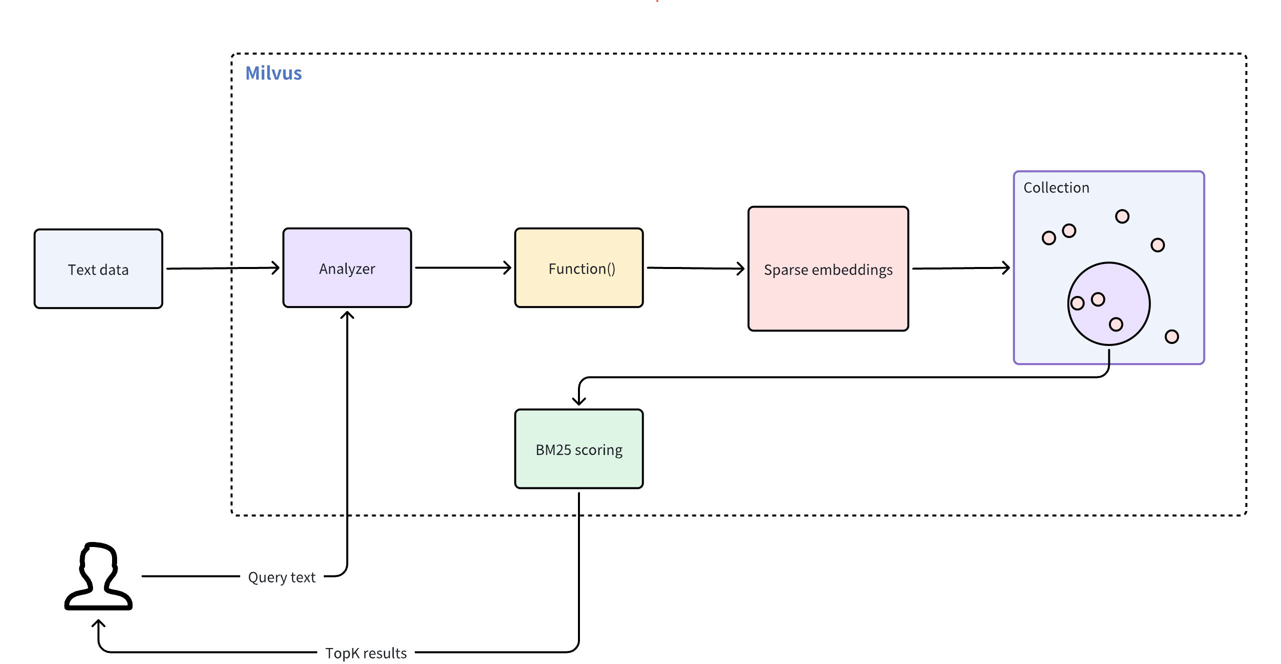
To use full text search, follow these main steps:
- Create a collection: Set up a collection with necessary fields and define a function to convert raw text into sparse embeddings.
- Insert data: Ingest your raw text documents to the collection.
- Perform searches: Use query texts to search through your collection and retrieve relevant results.
# Create a collection for full text search
To enable full text search, create a collection with a specific schema. This schema must include three necessary fields:
- The primary field that uniquely identifies each entity in a collection.
- A
VARCHARfield that stores raw text documents, with theenable_analyzerattribute set toTrue. This allows Milvus to tokenize text into specific terms for function processing. - A
SPARSE_FLOAT_VECTORfield reserved to store sparse embeddings that Milvus will automatically generate for theVARCHARfield.
# Define the collection schema
First, create the schema and add the necessary fields:
from pymilvus import MilvusClient, DataType, Function, FunctionType
client = MilvusClient(
uri="http://localhost:19530",
token="root:Milvus"
)
schema = client.create_schema()
schema.add_field(field_name="id", datatype=DataType.INT64, is_primary=True, auto_id=True)
schema.add_field(field_name="text", datatype=DataType.VARCHAR, max_length=1000, enable_analyzer=True)
schema.add_field(field_name="sparse", datatype=DataType.SPARSE_FLOAT_VECTOR)
2
3
4
5
6
7
8
9
10
11
12
In this configuration,
id: serves as the primary key and is automatically generated withauto_id=True.text: stores your raw text data for full text search operations. The data type must beVARCHAR, asVARCHARis Milvus string data type for text storage. Setenable_analyzer=Trueto allow Milvus to tokenize the text. By default, Milvus uses thestandardanalyzer for text analysis. To configure a different analyzer, refer to Analyzer Overview.sparse: a vector field reserved to store internally generated sparse embeddings for full text search operations. The data must beSPARSE_FLOAT_VECTOR.
Now, define a function that will convert your text into sparse vector representations and then add it to the schema:
bm25_function = Function(
name="text_bm25_emb", # Function name
input_field_names=["text"], # Name of the VARCHAR field containing raw text data
output_field_names=["sparse"], # Name of the SPARSE_FLOAT_VECTOR field reserved to store generated embeddings
function_type=FunctionType.BM25, # Set to BM25
)
schema.add_function(bm25_function)
2
3
4
5
6
7
8
| Parameter | Description |
|---|---|
name | The name of the function. This function converts your raw text from the text field into searchable vectors that will be stored in the sparse field. |
input_field_name | The name of the VARCHAR field requiring text-to-sparse-vector conversion. For FunctionType.BM25, this parameter accepts only one field name. |
output_field_name | The name of the field where the internally generated sparse vectors will be stored. For FunctionType.BM25, this parameter accepts only one field name. |
function_type | The type of the function to use. Set the value to FunctionType.BM25 |
NOTE
For collections with multiple VARCHAR fields requiring text-to-sparse-vector conversion, add separate functions to the collection schema, ensuring each function has a unique name and output_field_names value.
# Configure the index
After defining the schema with necessary fields and the built-in function, set up the index for your collection. To simplify this process, use AUTOINDEX as the index_type, an option that allows Milvus to choose and configure the most suitable index type based on the structure of your data.
index_params = client.prepare_index_params()
index_params.add_index(
field_name="sparse",
index_type="SPARSE_INVERTED_INDEX",
metric_type="BM25",
params={
"inverted_index_algo": "DAAT_MAXSCORE",
"bm25_k1": 1.2,
"bm25_b": 0.75
}
)
2
3
4
5
6
7
8
9
10
11
12
13
| Parameter | Description |
|---|---|
field_name | The name of the vector field to index. For full text search, this should be the field that stores the generated sparse vectors. In this example, set the value to sparse. |
index_type | The type of the index to create. AUTOINDEX allows Milvus to automatically optimize index settings. If you need more control over your index settings, you can choose from various index types available for sparse vectors in Milvus. For more information, refer to Indexes supported in Milvus |
metric_type | The value for this parameter must be set to BM25 specifically for full text search functionality. |
params | A dictionary of additional parameters specific to the index. |
params.inverted_index_algo | The algorithm used for building and querying the index. Valid values: 1. "DAAT_MAXSCORE" (default): Optimized Document-at-a-Time (DAAT) query processing using the MaxScore algorithm. MaxScore provides better performance for high k values or queries with many terms by skipping terms and documents likely to have minimal impact. It achieves this by partitioning terms into essential and non-essential groups based on their maximum impact scores, focusing on terms that can contribute to the top-k results. 2. "DAAT_WAND": Optimized DAAT query processing using the WAND algorithm. WAND evaluates fewer hit documents by leveraging maximum impact scores to skip noncompetitive documents, but it has a higher perhit overhead. This makes WAND more efficient for queries with small k values or short queries, where skipping is more feasible. 3. "TAAT_NAIVE": Basic Term-at-a-Time (TAAT) query processing. While it is slower compared to DAAT_MAXSCORE and DAAT_WAND, TAAT_NAIVE offers a unique advantage. Unlike DAAT algorithms, which use cached maximum impact scores that remain static regardless of changes to the global collection parameter (avgdl), TAAT_NAIVE dynamically adpats to such changes. |
params.bm25_k1 | Controls the term frequency saturation. Higher values increase the importance of term frequencies in document ranking. Value range: [1.2, 2.0]. |
params.bm25_b | Controls the extend to which document length is normalized. Values between 0 and 1 are typically used, with a common default around 0.75. A value of 1 means no length normalization, while a value of 0 means full normalization. |
# Create the collection
Now create the collection using the schema and index parameters defined.
client.create_collection(
collection_name='my_collection',
schema=schema,
index_params=index_params
)
2
3
4
5
# Insert text data
After setting up your collection and index, you're ready to insert text data. In this process, you need only to provide the raw text. The built-in function we defined earlier automatically generates the corresponding sparse vector for each text entry.
client.insert('my_collection', [
{'text': 'information retrieval is a field of study.'},
{'text': 'information retrieval focuses on finding relevant information in large datasets.'},
{'text': 'data mining and information retrieval overlap in research.'},
])
2
3
4
5
# Perform full text search
Once you've inserted data into your collection, you can perform full text searches using raw text queries. Milvus automatically converts your query into a sparse vector and ranks the matched search results using the BM25 algorithm, and then returns the topK (limit) results.
search_params = {
'params': {'drop_ratio_search': 0.2},
}
client.search(
collection_name='my_collection',
data=['whats the focus of information retrieval?'],
anns_field='sparse',
output_field=['text'], # Fields to return in search results; sparse field cannot be output
limit=3,
search_params=search_params
)
2
3
4
5
6
7
8
9
10
11
12
| Parameter | Description |
|---|---|
search_params | A dictionary containing search parameters. |
params.drop_ratio_search | Proportion of low-importance terms to ignore during search. For details, refer to Sparse Vector. |
data | Raw query text in natural language. Milvus automatically converts your text query into sparse vectors using the BM25 function - do not provide pre-computed vectors. |
anns_field | The name of the field that contains internally generated sparse vectors. |
output_fields | List of field names to return in search results. Supports all fields except the sparse vector field containing BM25-generated embeddings. Common output fields include the primary key field (e.g., id) and the original text field (e.g., text). For more information, refer to FAQ. |
limit | Maximum number of top matches to return. |
# FAQ
# Can I output or access the sparse vectors generated by the BM25 function in full text search?
No, the sparse vectors generated by the BM25 function are not directly accessible or outputable in full text search. Here are the details:
- The BM25 function generates sparse vectors internally for ranking and retrieval
- These vectors are stored in the sparse fields but cannot be included in
output_fields - You can only output the original text fields and metadata (like
id,text)
Example:
# ❌ This throws an error - you cannot output the sparse field
client.search(
collection_name='my_collection',
data=['query text'],
anns_field='sparse',
output_fields=['text', 'sparse'], # 'sparse' causes an error
limit=3,
search_params=search_params
)
# ✅ This works - output text files only
client.search(
collection_name='my_collection' ,
data=['query text'],
anns_field='sparse',
output_field=['text'],
limit=3,
search_params=search_params
)
2
3
4
5
6
7
8
9
10
11
12
13
14
15
16
17
18
19
# Why do I need to define a sparse vector field if I can't access it?
The sparse vector field serves as an internal search index, similar to database indexes that users don't directly interact with.
Design Rationale:
- Separation of concerns: You work with text (input/output), Milvus handles vectors (internal processing)
- Performance: Pre-computed sparse vectors enable fast BM25 ranking during queries
- User Experience: Abstracts away complex vector operations behind a simple text interface
If you need vector access:
- Use manual sparse vector operations instead of full text search
- Create separate collections for custom sparse vector workflows.
For details, refer to Sparse Vector.
# Text Match
Text match in Milvus enables precise document retrieval based on specific terms. This features is primarily used for filtered search to satisfy specific conditions and can incorporate scalar filtering to refine query results, allowing similarity searches within vectors that meet scalar criteria.
NOTE
Text match focuses on finding exact occurrences of the query terms, without scoring the relevance of the matched documents. If you want to retrieve the most relevant documents based on the semantic meaning and importance of the query terms, we recommend you use Full Text Search.
# Overview
Milvus integrates Tantivy to power its underlying inverted index and term-based text search. For each text entry, Milvus indexes it following the procedure:
- Analyzer: The analyzer processes input text by tokenizing it into individual words, or tokens, and then applying filters as needed. This allows Milvus to build an index based on these tokens.
- Indexing: After text analysis, Milvus creates an inverted index that maps each unique token to the documents containing it.
When a user performs a text match, the inverted index is used to quickly retrieve all documents containing the terms. This is much faster than scanning through each document individually.
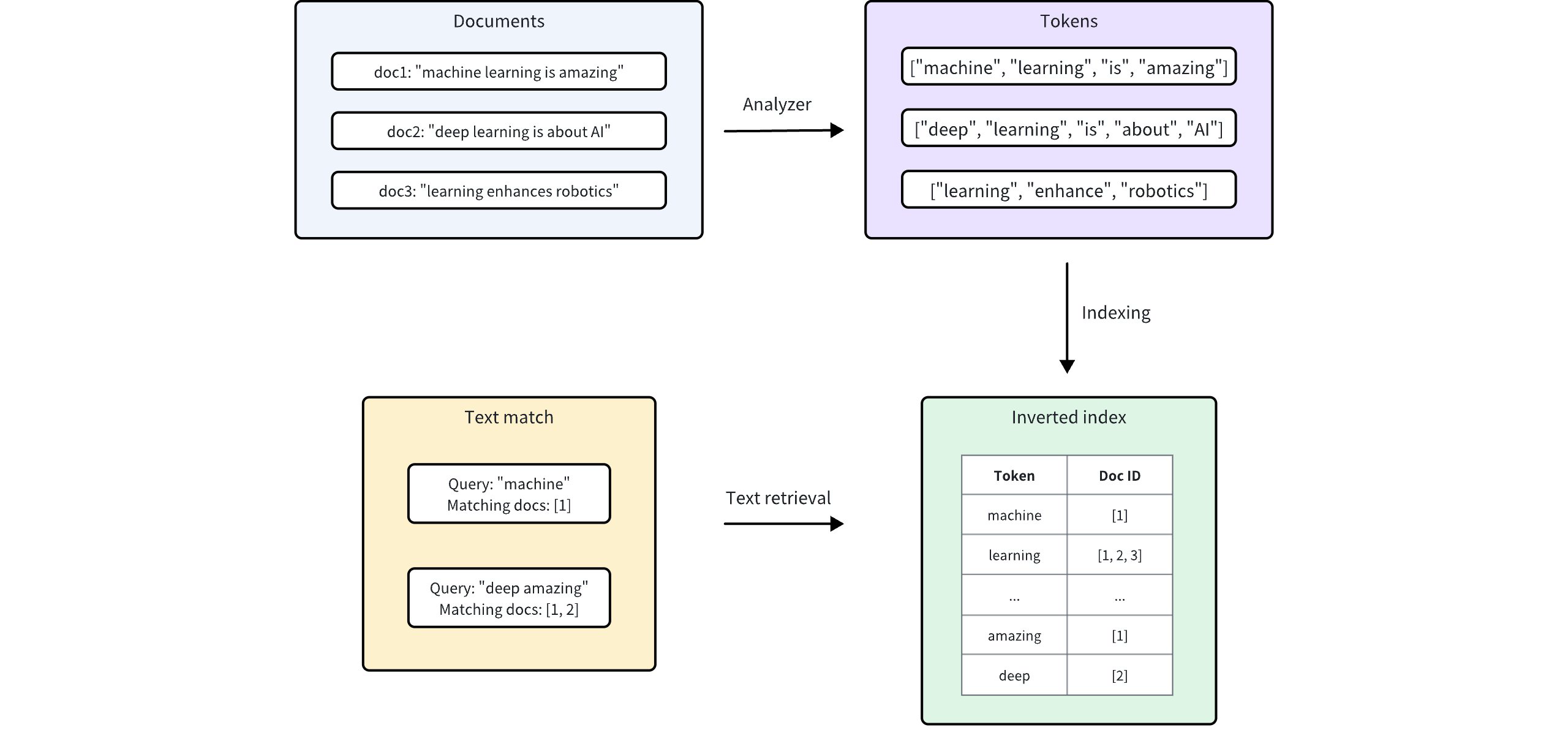
# Enable text match
Text match works on the VARCHAR field type, which is essentially the string data type in Milvus. To enable text match, set both enable_analyzer and enable_match to True and then optionally configure an analyzer for text analysis when defining your collection schema.
# Set enable_analyzer and enable_match
To enable text match for a specific VARCHAR field, set both the enable_analyzer and enable_match parameters to True when defining the field schema. This instructs Milvus to tokenize text and create an inverted index for the specified field, allowing fast and efficient text matches.
from pymilvus import MilvusClient, DataType
schema = MilvusClient.create_schema(enable_dynamic_field=False)
schema.add_field(
field_name="id",
datatype=DataType.INT64,
is_primary=True,
auto_id=True
)
schema.add_field(
field_name='text',
datatype=DataType.VARCHAR,
max_length=1000,
enable_analyzer=True, # Whether to enable text analysis for this field
enable_match=True # Whether to enable text match
)
schema.add_field(
field_name="embeddings",
datatype=DataType.FLOAT_VECTOR,
dim=5
)
2
3
4
5
6
7
8
9
10
11
12
13
14
15
16
17
18
19
20
21
# Optional: Configure an analyzer
The performance and accuracy of keyword matching depend on the selected analyzer. Different analyzers are tailored to various languages and text structures, so choosing the right one can significantly impact search results for your specific use case.
By default, Milvus uses the standard analyzer, which tokenizes text based on whitespace and punctuation, removes tokens longer than 40 characters, and converts text to lowercase. No additional parameters are needed to apply this default setting. For more information, refer to Standard.
In cases where a different analyzer is required, you can configure one using the analyzer_params parameter. For example, to apply the english analyzer for processing English text:
analyzer_params = {
"type": "english"
}
schema.add_field(
field_name='text',
datatype=DataType.VARCHAR,
max_length=200,
enable_analyzer=True,
analyzer_params=analyzer_params,
enable_match=True
)
2
3
4
5
6
7
8
9
10
11
Milvus also provides various other analyzers suited to different languages and scenarios. For more details, refer to Analyzer Overview.
# Use text match
Once you have enabled text match for a VARCHAR field in your collection schema, you can perform text matches using the TEXT_MATCH expression.
# TEXT_MATCH expression syntax
The TEXT_MATCH expression is used to specify the field and the terms to search for. Its syntax is as follows:
TEXT_MATCH(field_name, text)
field_name: The name of the VARCHAR field to search for.text: The terms to search for. Multiple terms can be separated by spaces or other appropriate delimiters based on the language and configured analyzer.
By default, TEXT_MATCH uses the OR matching logic, meaning it will return documents that contain any of the specified terms. For example, to search for documents containing the term machine or deep in the text field, use the following expression:
filter = "TEXT_MATCH(text, 'machine deep')"
You can also combine multiple TEXT_MATCH expressions using logical operators to perform AND matching.
- To search for documents containing both
machineanddeepin thetextfield, use the following expression:
filter = "TEXT_MATCH(text, 'machine') and TEXT_MATCH(text, 'deep')"
- To search for documents containing both
machineandlearningbut withoutdeepin thetextfield, use the following expressions:
filter = "not TEXT_MATCH(text, 'deep') and TEXT_MATCH(text, 'machine') and TEXT_MATCH(text, 'learning')"
# Search with text match
Text match can be used in combination with vector similarity search to narrow the search scope and improve search performance. By filtering the collection using text match before vector similarity search, you can reduce the number of documents that need to be searched, resulting in faster query times.
In this example, the filter expression filters the search results to only include documents that match the specified term keyword1 or keyword2. The vector similarity search is then performed on this filtered subset of documents.
# Match entities with `keyword1` or `keyword2`
filter = "TEXT_MATCH(text, 'keyword1 keyword2')"
# Assuming 'embeddings' is the vector field and 'text' is the VARCHAR field
result = client.search(
collection_name="my_collection", # Your collection name
anns_field="embeddings", # Vector field name
data=[query_vector], # Query vector
filter=filter,
search_params={"params": {"nprobe": 10}},
limit=10, # Max number of results to return
output_fields=["id", "text"] # Fields to return
)
2
3
4
5
6
7
8
9
10
11
12
13
# Query with text match
Text match can also be used for scalar filtering in query operations. By specifying a TEXT_MATCH expression in the expr parameter of the query() method, you can retrieve documents that match the given terms.
The example below retrieves documents where the text field contains both terms keyword1 and keyword2.
# Match entities with both `keyword1` and `keyword2`
filter = "TEXT_MATCH(text, 'keyword1') and TEXT_MATCH(text, 'keyword2')"
result = client.query(
collection_name="my_collection",
filter=filter,
output_fields=["id", "text"]
)
2
3
4
5
6
7
8
# Considerations
- Enabling term matching for a field triggers the creation of an inverted index, which consumes storage resources. Consider storage impact when deciding to enable this feature, as it varies based on text size, unique tokens, and the analyzer used.
- Once you've defined an analyzer in your shcema, its settings become permanent for that collection. If you decide that a different analyzer would better suit your needs, you may consider dropping the existing collection and creating a new one with the desired analyzer configuration.
- Escape rules in
filterexpressions:- Characters enclosed in double quotes or single quotes within expressions are interpreted as string constants. If the string constant includes characters, the escape characters must be represented with escape sequence. For example, use
\\to represent\,\\tto represent a tab\t, and\\nto represent a newline. - If a string constant is enclosed by single quotes, a single quote within the constant should be represented as
\\'while a double quote can be represented as either"or\\". Example:'It\\'s milvus'. - If a string constant is enclosed by double quotes, a double quote within the constant should be represented as
\\"while a single quote can be represented as either'or\\'. Example:"He said \\"Hi\\"".
- Characters enclosed in double quotes or single quotes within expressions are interpreted as string constants. If the string constant includes characters, the escape characters must be represented with escape sequence. For example, use
# Phrase Match
Phrase match lets you search for documents containing your query terms as an exact phrase. By default, the words must apear in the same order and directly adjacent to one another. For example, a query for "robotics machine learning" matches text like "...typical robotics machine learning models...", where the words "robotics", "machine", and "learning" apear in sequence with no other words between them.
However, in real-world scenarios, strict phrase matching can be too rigid. You might want to match text like "...machine learning models widely adopted in robotics...". Here, the same keywords are present but not side-by-side or in the original order. To handle this, phrase match supports a slop parameter, which introduces flexibility. The slop value defines how many positional shifts are allowed between the terms in the phrase. For example, with a slop of 1, a query for "maching learning" can match text like "...machine deep learning...", where one word ("deep") separates the original terms.
# Overview
Powered by the Tantivy search engine library, phrase match words by analyzing the positional information of words within documents. The diagram below illustrates the process:
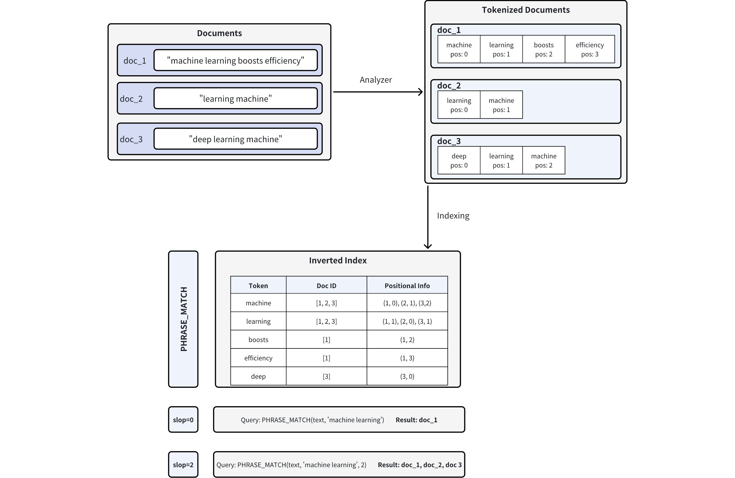
- Document Tokenization: When you insert documents into Milvus, the text is split into tokens (individual words or terms) using an analyzer, with positional information recorded for each token. For example, doc_1 is tokenized into ["machine" (pos=0), "learning" (pos=1), "boosts" (pos=2), "efficiency" (pos=3)]. For more information on analyzers, refer to Analyzer Overview.
- Inverted Index Creation: Milvus builds an inverted index, mapping each token to the document(s) in which it appears and the token's positions in those documents.
- Phrase Matching: When a phrase query is executed, Milvus looks up each token in the inverted index and checks their positions to determine if they appear in the correct order and proximity. The
slopparameter controls the maximum number of positions allowed between matching tokens:slop = 0means the tokens must appear in the exact order and immediately adjacent (i.e., no extra words in between).- In the example, only doc_1 ("machine" at pos=0, "learning" at pos=1) matches exactly.
slop = 2allows up to two positions of flexibility or rearrangements between matching tokens.- This allows reversed order ("learning machine") or a small gap between the tokens.
- Consequently, doc_1, doc_2 ("learning" at pos=0, "machine" at pos=1), and doc_3 ("learning" at pos=1, "machine" at pos=2) all match.
# Enable phrase match
Phrase match works with the VARCHAR field type, the string data type in Milvus. To enable phrase matching, configure your collection schema by setting both enable_analyzer and enable_match parameters to True, similar to text match.
# Set enable_analyzer and enable_match
To enable phrase match for a specific VARCHAR field, set both enable_analyzer and enable_match parameters to True when defining the field schema. This configuration instructs Milvus to tokenize the text and create an inverted index with positional information required for efficient phrase matching.
Here's an example schema definition to enable phrase match:
from pymilvus import MilvusClient, DataType
# Create a schema for a new collection
schema = MilvusClient.create_schema(enable_dynamic_field=False)
schema.add_field(
field_name="id",
datatype=DataType.INT64,
is_primary=True,
auto_id=True
)
# Add a VARCHAR field configured for phrase matching
schema.add_field(
field_name='text', # Name of the field
datatype=DataType.VARCHAR, # Field data type set as VARCHAR (string)
max_length=1000, # Maximum length of the string
enable_analyzer=True, # Enables text analysis (tokenization)
enable_match=True # Enables inverted indexing for phrase matching
)
schema.add_field(
field_name="embeddings",
datatype=DataType.FLOAT_VECTOR,
dim=5
)
2
3
4
5
6
7
8
9
10
11
12
13
14
15
16
17
18
19
20
21
22
23
24
# Optional: Configure an analyzer
Phrase matching accuracy depends significantly on the analyzer used to tokenize your text data. Different analyzers suit different languages and text formats, affecting tokenization and positional accuracy. Selecting an appropriate analyzer for your specific use case will optimize your phrase matching results.
By default, Milvus uses the standard analyzer, which tokenizes text based on whitespace and punctuation, removes tokens longer than 40 characters, and converts text to lowercase. No additional parameters are required for default usage. Refer to Standard Analyzer for details.
If your application requires a specific analyzer, configure it using the analyzer_params parameter. For example, here's how to configure the english analyzer for phrase matching in English text:
# Define analyzer parameters for English-language tokenization
analyzer_params = {
"type": "english"
}
# Add the VARCHAR field with the English analyzer enabled
schema.add_field(
field_name='text', # Name of the field
datatype=DataType.VARCHAR, # Field data type set as VARCHAR
max_length=1000, # Maximum length of the string
enable_analyzer=True, # Enables text analysis
analyzer_params=analyzer_params, # Specifies the analyzer configuration
enable_match=True # Enables inverted indexing for phrase matching
)
2
3
4
5
6
7
8
9
10
11
12
13
14
Milvus supports several analyzers tailored for different languages and use cases. For detailed information, refer to Analyzer Overview.
# Use phrase match
Once you've enabled match for a VARCHAR field in your collection schema, you can perform phrase matches using the PHRASE_MATCH expression.
NOTE
The PHRASE_MATCH expression is case-insensitive. You can use either PHRASE_MATCH or phrase_match.
# PHRASE_MATCH expression syntax
Use the PHRASE_MATCH expression to specify the field, phrase, and optional flexibility (slop) when searching. The syntax is:
PHRASE_MATCH(field_name, phrase, slop)
field_name: The name of theVARCHARfield on which you perform phrase matches.phrase: The exact phrase to search for.slop(optional): An integer specifying the maximum number of positions allowed in matching tokens.0(default): Matches exact phrases only. Example: A filter for "maching learning" will match "maching learning" exactly, but not "machine boosts learning" or "learning machine".1: Allows minor variation, such as one extra term or minor shift in position. Example: A filter for "machine learning" will match "machine boosts learning" (one token between "machine" and "learning") but not "learning machine" (terms reversed).2: Allows more flexibility, including reversed term order or up to two tokens in between. Example: A filter for "machine learning" will match "learning machine" (terms reversed) or "machine quickly boosts learning" (two tokens between "machine" and "learning").
# Example dataset
Suppose you have a collection named tech_articles containing the following five entities:
doc_id | text |
|---|---|
| 1 | "Machine learning boosts efficiency in large-scale data analysis" |
| 2 | "Learning a machine-based approach is vital for modern AI progress" |
| 3 | "Deep learning machine architectures optimize computational loads" |
| 4 | "Machine swiftly improves model performance for ongoing learning" |
| 5 | "Learning advanced machine algorithms expands AI capabilities" |
# Query with phrase match
When using the query() method, PHRASE_MATCH acts as a scalar filter. Only documents that contain the specified phrase (subject to the allowed slop) are returned.
Example: slop=0 (exact match): This example returns documents containing the exact phrase "machine learning" without any extra tokens in between.
# Match documents containing exactly "machine learning"
filter = "PHRASE_MATCH(text, 'machine learning')"
result = client.query(
collection_name="tech_articles",
filter=filter,
output_fields=["id", "text"]
)
2
3
4
5
6
7
8
Expected match results:
doc_id | text |
|---|---|
| 1 | "Machine learning boosts efficiency in large-scale data analysis" |
Only document 1 contains the exact phrase "machine learning" in the specified order with no additional tokens.
# Search with phrase match
In search operations, PHRASE_MATCH is used to filter documents before applying vector similarity ranking. This two-step approach first narrows the candidate set by textuall matching and then re-ranks those candidates based on vector embeddings.
Example: slop=1: Here, we allow a slop of 1. The filter is applied to documents that contain the phrase "learning machine" with slight flexibility.
# Example: Filter documents containing "learning machine" with slop=1
filter_slop1 = "PHRASE_MATCH(text, 'learning machine', 1)"
result_slop1 = client.search(
collection_name="tech_articles",
anns_field="embeddings",
data=[query_vector],
filter=filter_slop1,
search_params={"params": {"nprobe": 10}},
limit=10,
output_fields=["id", "text"]
)
2
3
4
5
6
7
8
9
10
11
12
Match results:
doc_id | text |
|---|---|
| 2 | "Learning a machine-based approach is vital for modern AI progress" |
| 3 | "Deep learning machine architectures optimize computational loads** |
| 5 | "Learning advanced machine algorithms expands AI capabilities" |
Example: slop=2: This example allows a slop of 2, meaning that up to two extra tokens (or reversed terms) are allowed between the words "machine" and "learning".
filter_slop2 = "PHRASE_MATCH(text, 'machine learning', 2)"
result_slop2 = client.search(
collection_name="tech_articles",
anns_field="embeddings", # Vector field name
data=[query_vector], # Query vector
filter=filter_slop2, # Filter expression
search_params={"params": {"nprobe": 10}},
limit=10, # Maximum results to return
output_fields=["id", "text"]
)
2
3
4
5
6
7
8
9
10
11
Match results:
doc_id | text |
|---|---|
| 1 | "Machine learning boosts efficiency in large-scale data analysis" |
| 3 | "Deep learning machine architectures optimize computational loads" |
Example: slop=3: In this example, a slop of 3 provides even more flexibility. The filter searches for "machine learning" with up to three token positions allowed between the words.
filter_slop3 = "PHRASE_MATCH(text, 'machine learning', 3)"
result_slop2 = client.search(
collection_name="tech_articles",
anns_field="embeddings", # Vector field name
data=[query_vector], # Query vector
filter=filter_slop3, # Filter expression
search_params={"params": {"nprobe": 10}},
limit=10, # Maximum results to return
output_fields=["id", "text"]
)
2
3
4
5
6
7
8
9
10
11
Match results:
doc_id | text |
|---|---|
| 1 | "Machine learning boosts efficiency in large-scale data analysis" |
| 2 | "Learning a machine-based approach is vital for modern AI progress" |
| 3 | "Deep learning machine architectures optimize computational loads" |
| 5 | "Learning advanced machine algorithms expands AI capabilities" |
# Considerations
- Enabling phrase matching for a field triggers the creation of an inverted index, which consumes storage resources. Consider storage impact when deciding to enable this feature, as it varies based on text size, unique tokens, and the analyzer used.
- Once you've defined an analyzer in your shcema, its settings become permanent for that collection. If you decide that a different analyzer would better suit your needs, you may consider dropping the existing collection and creating a new one with the desired analyzer configuration.
- Escape rules in
filterexpressions:- Characters enclosed in double quotes or single quotes within expressions are interpreted as string constants. If the string constant includes characters, the escape characters must be represented with escape sequence. For example, use
\\to represent\,\\tto represent a tab\t, and\\nto represent a newline. - If a string constant is enclosed by single quotes, a single quote within the constant should be represented as
\\'while a double quote can be represented as either"or\\". Example:'It\\'s milvus'. - If a string constant is enclosed by double quotes, a double quote within the constant should be represented as
\\"while a single quote can be represented as either'or\\'. Example:"He said \\"Hi\\"".
- Characters enclosed in double quotes or single quotes within expressions are interpreted as string constants. If the string constant includes characters, the escape characters must be represented with escape sequence. For example, use
# Elasticsearch Queries to Milvus
Elasticsearch, built on Apache Lucene, is a leading open-source search engine. However, it faces chanllenges in modern AI applications, including high update costs, poor real-time performance, inefficient shard management, a non-cloud-native design, and excessive resource demands. As a cloud-native vector database, Milvus overcomes these issues with decoupled storage and computing, efficient indexing for high-dimensional data, and seamless integration with modern infrastructures. It offers superior performance and scalability for AI workloads.
This article aims to facilitate the migration of your code base from Elasticsearch to Milvus, providing various examples of converting queries in between.
# Overview
In Elasticsearch, operations in the query context generate relevance scores, while those in the filter context do not. Similarly, Milvus searches produce similarity scores, whereas its filter-like queries do not. When migrating your code base from Elasticsearch to Milvus, the key principle is converting fields used in Elasticsearch's query context into vector fields to enable similarity score generation.
The table below outlines some Elasticsearch query patterns and their corresponding equivalents in Milvus.
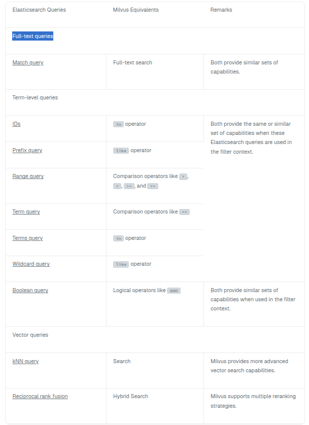
# Full-text queries
In Elasticsearch, the full text queries enable you to search analyzed text fields such as the body of the email. The query string is processed using the same analyzer that was applied to the field during indexing.
# Match query
In Elasticsearch, a match query returns documents that match a provided text, number, date, or boolean value. The provided text is analyzed before matching.
The following is an example Elasticsearch search request with a match query.
resp = client.search(
query={
"match": {
"message": {
"query": "this is a test"
}
}
}
)
2
3
4
5
6
7
8
9
Milvus provides the same capability throuhg the full-text search feature. You can convert the above Elasticsearch query into Milvus as follows:
res = client.search(
collection_name="my_collection",
data=['How is the weather in Jamaica?'],
anns_field="message_sparse",
output_fields=["id", "message"]
)
2
3
4
5
6
In the example above, message_sparse is a sparse vector field derived from a VarChar field named message. Milvus uses the BM25 embedding model to convert the values in the message field into sparse vector embeddings and stores them in the message_sparse field. Upon receiving the search request, Milvus embeds the plain text query payload using the same BM25 model and performs a sparse vector search and returns the id and message fields specified in the output_fields parameter along with the corresponding similarity scores.
To use this functionality, you must enable the analyzer on the message field and define a function to derive the message_sparse field from it. For detailed instructions on enabling the analyzer and creating the derivative function in Milvus, refer to Full Text Search.
# Term-level queries
In Elasticsearch, term-level queries are used to find documents based on exact values in structured data, such as date ranges, IP addresses, prices, or product IDs. This section outlines the possible equivalents of some Elasticsearch term-level queries in Milvus. All examples in this section are adapted to operate within the filter context to align with Milvus's capabilities.
# IDs
In Elasticsearch, you can find documents based on their IDs in the filter context as follows:
resp = client.search(
query={
"bool": {
"filter": {
"ids": {
"values": [
"1",
"4",
"100"
]
}
}
}
}
)
2
3
4
5
6
7
8
9
10
11
12
13
14
15
In Milvus, you can also find entities based on their IDs as follows:
# Use the filter parameter
res = client.query(
collection_name="my_collection",
filter="id in [1, 4, 100]",
output_fields=["id", "title"]
)
# Use the ids parameter
res = client.query(
collection_name="my_collection",
ids=[1, 4, 100],
output_fields=["id", "title"]
)
2
3
4
5
6
7
8
9
10
11
12
13
You can find the Elasticsearch example on this page. For details on query and get requests as well as the filter expressions in Milvus, refer to Query and Filtering.
# Prefix query
In Elasticsearch, you can find documents that contain a specific prefix in a provided field in the filter context as follows:
resp = client.search(
query={
"bool": {
"filter": {
"prefix": {
"user": {
"value": "ki"
}
}
}
}
}
)
2
3
4
5
6
7
8
9
10
11
12
13
In Milvus, you can find the entities whose values start with the specified prefix as follows:
res = client.query(
collection_name="my_collection",
filter='user like "ki%"',
output_fields=["id", "user"]
)
2
3
4
5
You can find the Elasticsearch example on this page. For details on the like operator in Milvus, refer to Using LIKE for Pattern Matching.
# Range query
In Elasticsearch, you can find documents that contain terms within a provided range as follows:
resp = client.search(
query={
"bool": {
"filter": {
"range": {
"age": {
"gte": 10,
"lte": 20
}
}
}
}
}
)
2
3
4
5
6
7
8
9
10
11
12
13
14
In Milvus, you can find the entities whose values in a specific field are within a provided range as follows:
res = client.query(
collection_name="my_collection" ,
filter='10 <= age <= 20',
output_fields=["id", "user", "age"]
)
2
3
4
5
You can find the Elasticsearch example on this page. For details on comparison operators in Milvus, see Comparison operators.
# Term query
In Elasticsearch, you can find documents that contain an exact term in a provided field as follows:
resp = client.search(
query={
"bool": {
"filter": {
"term": {
"status": {
"value": "retired"
}
}
}
}
}
)
2
3
4
5
6
7
8
9
10
11
12
13
In Milvus, you can find the entities whose values in the specified field are exactly the specified term as follows:
# use ==
res = client.query(
collection_name="my_collection",
filter='status == "retired"',
output_fields=["id", "user", "status"]
)
# use TEXT_MATCH
res = client.query(
collection_name="my_collection",
filter='TEXT_MATCH(status, "retired")',
output_fields=["id", "user", "status"]
)
2
3
4
5
6
7
8
9
10
11
12
13
You can find the Elasticsearch example on this page. For details on comparison operators in Milvus, see Comparison operators.
# Terms query
In Elasticsearch, you can find documents that contain one or more exact terms in a provided field as follows:
resp = client.search(
query={
"bool": {
"filter": {
"terms": {
"degree": [
"graduate",
"post-graduate"
]
}
}
}
}
)
2
3
4
5
6
7
8
9
10
11
12
13
14
Milvus does not have a complete equivalence of this one. However, you can find the entities whose values in the specified field are one of the specified terms as follows:
# use in
res = client.query(
collection_name="my_collection",
filter='degree in ["graduate", "post-graduate"]',
output_field=["id", "user", "degree"]
)
# use TEXT_MATCH
res = client.query(
collection_name="my_collection",
filter='TEXT_MATCH(degree, "graduate post-graduate")',
output_fields=["id", "user", "degree"]
)
2
3
4
5
6
7
8
9
10
11
12
13
You can find the Elasticsearch example on this page. For details on range operators in Milvus, refer to Range operators.
# Wildcard query
In Elasticsearch, you can find documents that contain terms matching a wildcard pattern as follows:
res = client.search(
query={
"bool": {
"filter": {
"wildcard": {
"user": {
"value": "ki*y"
}
}
}
}
}
)
2
3
4
5
6
7
8
9
10
11
12
13
Milvus does not support wildcard in its filtering conditions. However, you can use the like operator to achieve the similar effect as follows:
res = client.query(
collection_name="my_collection",
filter='user like "ki%" AND user like "%y"' ,
output_fields=["id", "user"]
)
2
3
4
5
You can find the Elasticsearch example on this page. For details on the range operators in Milvus, refer to Range operators.
# Boolean query
In Elasticsearch, a boolean query is a query that matches documents matching boolean combinations of other queries.
The following example is adapted from an example in Elasticsearch documentation on this page. The query will return users with kimchy in their names with a production tag.
resp = client.search(
query={
"bool": {
"filter": {
"term": {
"user": "kimchy"
}
},
"filter": {
"term": {
"tags": "production"
}
}
}
}
)
2
3
4
5
6
7
8
9
10
11
12
13
14
15
16
In Milvus, you can do the similar thing as follows:
res = client.query(
collection_name="my_collection",
filter='user like "%kimchy%" AND ARRAY_CONTAINS(tags, "production")',
output_fields=["id", "user", "age", "tags"]
)
2
3
4
5
The above example assumes that you have a user field of the VarChar type and a tags field of the Array type, in the target collection. The query will return users with kimchy in their names with a production tag.
# Vector queries
In Elasticsearch, vector queries are specialized queries that work on vector fields to efficiently perform semantic search.
# Knn query
Elasticsearch supports both approximate kNN queries and exact, brute-force kNN queries. You can find the k nearest vectors to a query vector in either way, as measured by a similarity metric, as follows:
resp = client.search(
index="my-image-index" ,
size=3,
query={
"knn": {
"field": "image-vector",
"query_vector": [
-5,
9,
-12
],
"k": 10
}
}
)
2
3
4
5
6
7
8
9
10
11
12
13
14
15
Milvus, as a specialized vector database, uses index types to optimize vector searches. Typically, it prioritizes approximate nearest neighbor (ANN) search for high-dimensional vector data. While brute-force kNN search with the FLAT index type delivers precise results, it it both time-consuming and resource-intensive. In contrast, ANN search using AUTOINDEX or other index types balances speed and accuracy, offering significantly faster and more resource-efficient performance than kNN.
A similar equivalence to the above vector query in Milvus goes like this:
res = client.search(
collection_name="my_collection" ,
anns_field="image-vector",
data=[[-5, 9, -12]],
limit=10
)
2
3
4
5
6
You can find the Elasticsearch example on this page. For details on ANN searches in Milvus, read Basic ANN Search.
# Reciprocal Rank Fusion
Elasticsearch provides Reciprocal Rank Fusion (RRF) to combine multiple result sets with different relevance indicators into a single ranked result set.
The following example demonstrates combining a traditional term-based search with a k-nearest neighbors (kNN) vector search to improve search relevance:
client.search(
index="my_index" ,
size=10,
query={
"retriever": {
"rrf": {
"retrievers": [
{
"standard": {
"query": {
"term": {
"text": "shoes"
}
}
}
},
{
"knn": {
"field": "vector",
"query_vector": [1.25, 2, 3.5], # Example vector; replace with your actual query vector
"k": 50,
"num_candidates": 100
}
}
],
"rank_window_size": 50,
"rank_constant": 20
}
}
}
)
2
3
4
5
6
7
8
9
10
11
12
13
14
15
16
17
18
19
20
21
22
23
24
25
26
27
28
29
30
31
In this example, RRF combines results from two retrievers:
- A standard term-based search for documents containing the term "shoes" in the
textfield. - A kNN search on the
vectorfield using the provided query vector.
Each retriever contributes up to 50 top matches, which are reranked by RRF, and the final top 10 results are returned.
In Milvus, you can achieve a similar hybrid search by combining searches across multiple vector fields, applying a reranking strategy, and retrieving the top-K results from the combined list. Milvus supports both RRF and weighted reranker strategies. For more details, refer to Reranking.
The following is a non-strict equivalence of the above Elasticsearch examples in Milvus.
search_params_dense = {
"data": [[1.25, 2, 3.5]],
"anns_field": "vector",
"param": {
"metric_type": "IP",
"params": {"nprobe": 10},
},
"limit": 100
}
req_dense = ANNSearchRequest(**search_params_dense)
search_params_sparse = {
"data": ["shoes"],
"anns_field": "text_sparse",
"param": {
"metric_type": "BM25",
"params": {"drop_ratio_search": 0.2}
}
}
req_sparse = ANNSearchRequest(**search_params_sparse)
res = client.hybrid_search(
collection_name="my_collection",
reqs=[req_dense, req_sparse],
reranker=RRFRanker(),
limit=10
)
2
3
4
5
6
7
8
9
10
11
12
13
14
15
16
17
18
19
20
21
22
23
24
25
26
27
28
29
This example demonstrates a hybrid search in Milvus that combines:
- Dense vector search: Using the inner product (IP) metric with
nprobeset to 10 for approximate nearest neighbor (ANN) search on thevectorfield. - Sparse vector search: Using the BM25 similarity metric with a
drop_ratio_searchparameter of 0.2 on thetext_sparsefield.
The results from these searches are executed separately, combined, and reranked using the Reciprocal Rank Fusion (RRF) ranker. The hybrid search returns the top 10 entities from the reranked list.
Unlike Elasticsearch's RRF ranking, which merges results from standard text-based queries and kNN searches, Milvus combines results from sparse and dense vector searches, providing a unique hybrid search capability optimized for multimodal data.
# Recap
In this article, we covered the conversions of typical Elasticsearch queries to their Milvus equivalents, including term-level queries, boolean queries, full-text queries, and vector queries. If you have further questions about converting other Elasticsearch queries, feel free to reach out to us.
# Search Iterators
The ANN Search has a maximum limit on the number of entities that can be recalled in a single query, and simply using basic ANN Search may not meet the demands of large-scale retrieval. For ANN Search requests where topK exceeds 16384, it is advisable to consider using the SearchIterator. This section will introduce how to use the SearchIterator and related considerations.
# Overview
A Search request returns search results, while a SearchIterator returns an iterator. You can call the next() method of this iterator to get the search results.
Specifically, you can use the SearchIterators as follows:
- Create a SearchIterator and set the number of entities to return per search request and the total number of entities to return.
- Call the next() method of the SearchIterator in a loop to get the search result in a paginated manner.
- Call the close() method of the iterator to end the loop if the next() method returns an empty result.
# Create SearchIterator
The following code snippet demonstrates how to create a SearchIterator.
from pymilvus import connections, Collection
connections.connect(
uri="http://localhost:19530",
token="root:Milvus"
)
# create iterator
query vectors = [[0.3580376395471989, -0.6023495712049978, 0.18414012509913835, -0.26286205330961354, 0.9029438446296592]]
collection = Collection("iterator_collection")
iterator = collection.search_iterator(
data=query_vectors,
anns_field="vector",
param={"metric_type": "L2", "params": {"nprobe": 16}},
batch_size=50,
output_fields=["color"],
limit=20000
)
2
3
4
5
6
7
8
9
10
11
12
13
14
15
16
17
18
19
20
In the above examples, you have set the number of entities to return per search (batch_size/batchSize) to 50, and the total number of entities to return (topK) to 20000.
# Use SearchIterator
Once the SearchIterator is ready, you can call its next() method to get the search results in a paginated manner.
results = []
while True:
result = iterator.next()
if not result:
iterator.close()
break
for hit in result:
results.append(hit.to_dict())
2
3
4
5
6
7
8
9
10
In the above code examples, you have created an infinte loop and called the next() method in the loop to store the search results in a variable and closed the iterator when the next() returns nothing.
# Use Partition Key
# Embeddings & Reranking
# Storage Optimization
- Database
- What is a database
- Create database
- View database
- Manage database properties
- Use database
- Drop database
- FAQ
- Collections
- Collection Explained
- Create Collection
- View Collections
- Modify Collection
- Load & Release
- Set Collection TTL
- Set Consistency Level
- Manage Partitions
- Manage Aliases
- Drop Collection
- Schema & Data Fields
- Schema Explained
- Primary Field & AutoID
- Dense Vector
- Binary Vector
- Sparse Vector
- String Field
- Number Field
- JSON Field
- Array Field
- Dynamic Field
- Nullable & Default
- Analyzer
- Alter Collection Field
- Add Fields to an Existing Collection
- Insert & Delete
- Insert Entities
- Upsert Entities
- Delete Entities
- Indexes
- Index Explained
- Floating Vector Indexes
- Binary Vector Indexes
- Sparse Vector Indexes
- Scalar Indexes
- GPU-enabled Indexes
- Search
- Basic ANN Search
- Filtered Search
- Range Search
- Grouping Search
- Hybrid Search
- Query
- Filtering
- Full Text Search
- Text Match
- Phrase Match
- Elasticsearch Queries to Milvus
- Search Iterators
- Use Partition Key
- Embeddings & Reranking
- Storage Optimization